|
The progress of empirical sciences comes with the formulation and testing of new hypotheses, which are helpful for a clearer and deeper understanding of
phenomena. Often new strategies for practice can be derived from them. A hypothesis is considered as valid if it has been supported by empirical
data and until it is disproved by new empirical data. In fact, a hypothesis can never be fully proved. |
|
Educational objectives
After having worked through this chapter you will know the structure of a statistical hypothesis test, the various test decisions, the errors that can be made, the probabilities of these errors, as well as the relation between these terms. You will furthermore know how to formulate the null hypothesis and the alternative hypothesis for a test situation. Key words: null hypothesis, alternative hypothesis, test statistic, rejection region of \( H_0 \), type I error, \( \alpha \)-error probability, significance level, type II error, \( \beta \)-error probability, statistical power, \( p \)-value Previous knowledge: nominal data, quantitative data (chap. 1), sample, mean value (chap. 3), normal distribution (chap. 6), sampling distribution (chap. 8) Central questions: What is a statistical hypothesis test? What does the result of a statistical hypothesis test mean? Which errors can be made in such a test? How can these errors be controlled? |
Do women eat too little before their menstruation?

It is suspected that the daily energy consumption of women before their menstruation lies under a recommended value of \( 7425 \text{kJ} \). In a study by Manocha et al. (1986) (cf. [1], page 188), the average daily energy consumption was recorded for a period of 10 days among 11 randomly chosen healthy women aged between 20 and 30 years prior to their menstruation. The following values in kJ/day were measured in this study: \[ 5260, 5470, 5640, 6180, 6390, 6515, 6805, 7515, 7515, 8230, 8770 \text{ kJ} .\]
The 11 women had an average consumption of \( 6753.6 \text{kJ} \) per day. We already know from chapter 8, that the sample mean represents a random value. Can we now state, based on this sample, that the mean energy consumption prior to the menstruation phase, (\( \mu \)), in a population of healthy women between 20 and 30 years of age is indeed lower than the recommended value? In order to answer this and similar questions, the concept of statistical hypothesis testing was introduced.
If we have the impression that the mean daily energy consumption \( \mu \) in the population of women in the pre-menstruation phase lies under the recommended value of \( 7425 \text{ kJ} \), and if we want to see whether the data support this assumption, we formulate the assumption in the hypothesis \( H_A: \mu \lt 7425 \text{kJ} \).
The converse hypothesis will be that the mean energy consumption in this sub-population of women is \( \geq 7425 \text{ kJ} \). This hypothesis is called the null hypothesis (\(H_0\)).It would be natural to consider our own hypothesis as the primary one and the null hypothesis as the "alternative hypothesis". However, we will see that the null hypothesis plays a fundamental role in deciding whether \( H_A \) is sufficiently supported by the observed data or not. This is why \( H_0 \) is considered the "point of departure" from a theoretical perspective, while the researchers' hypothesis represents the alternative to the null hypothesis.
|
Definition 9.1.1
In the alternative hypothesis \( H_A \), we postulate
|
|
Synopsis 9.1.1
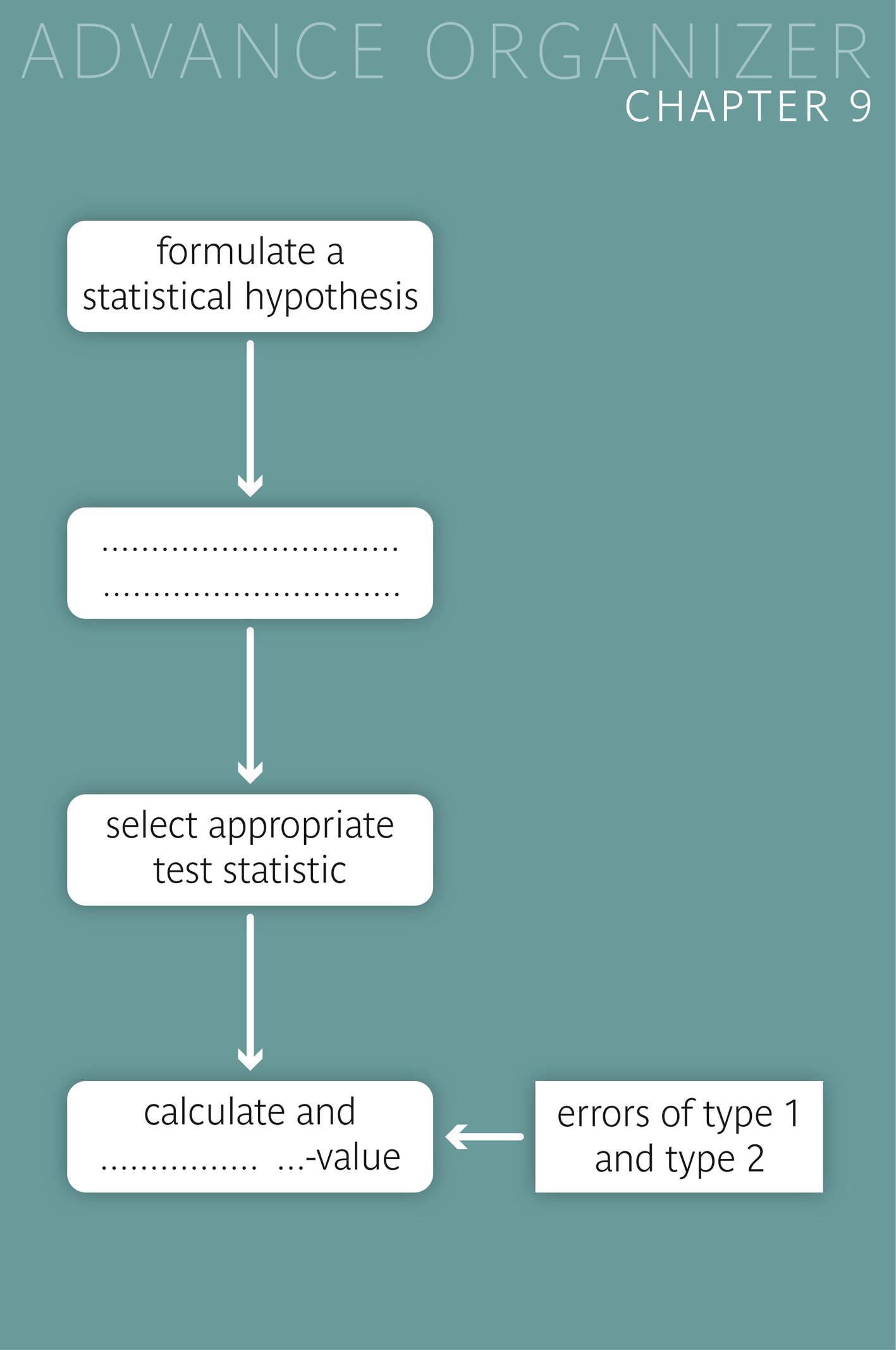
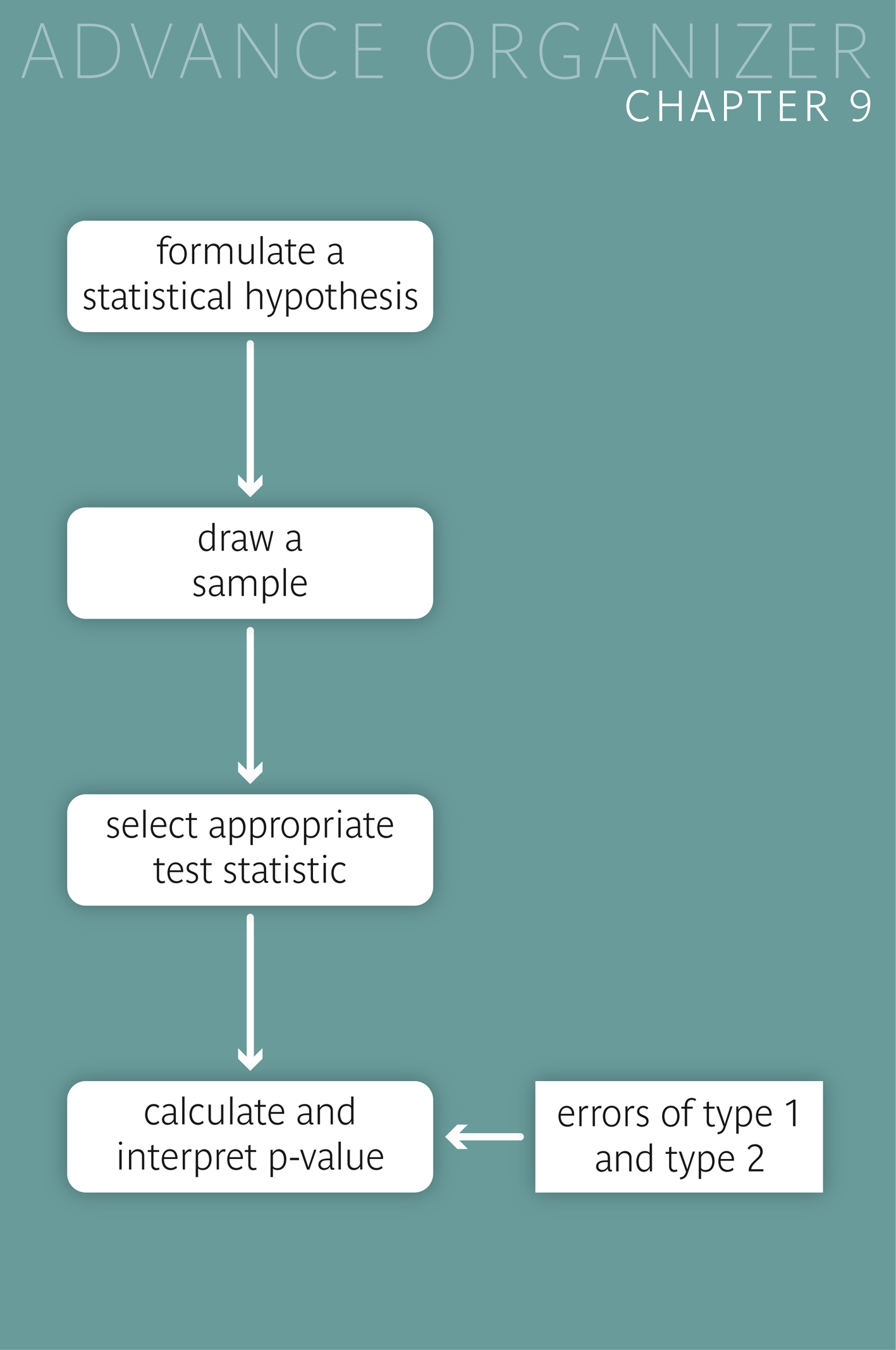
Tn a first step we phrase our hypothesis \( H_A \) and the null-hypothesis \( H_0 \). In a second step, we collect appropriate data for testing \( H_A \). In our example, we have
with \( \mu \) denoting the unknown mean daily energy uptake of women before their menstruation. |
In our example, we can use the observed mean value of the energy consumption as a test statistic in order to decide whether to reject the null hypothesis \( H_0 : \mu \geq 7425 \text{ kJ} \) (and hence decide in favor of the alternative hypothesis) or not. The value of our test statistic, namely \( 6753.6 \text{ kJ} \), rather seems to speak in favour of \( H_A : \mu \lt 7425 \text{ kJ} \). But if we had observed a sample mean of \( 6000 \text{ kJ} \) in another sample of 11 women, this would speak even more strongly in favour of\( H_A \) than the value \( 6753.6 \text{ kJ} \).
|
Definition 9.1.2
A test statistic is a measure, which is calculated from a sample according to a given rule and which is suitable to test an alternative hypothesis. |
|
Synopsis 9.1.2
After having formulated the null- and the alternative hypothesis, we calculate a test statistic which is suitable for testing the given alternative hypothesis. |
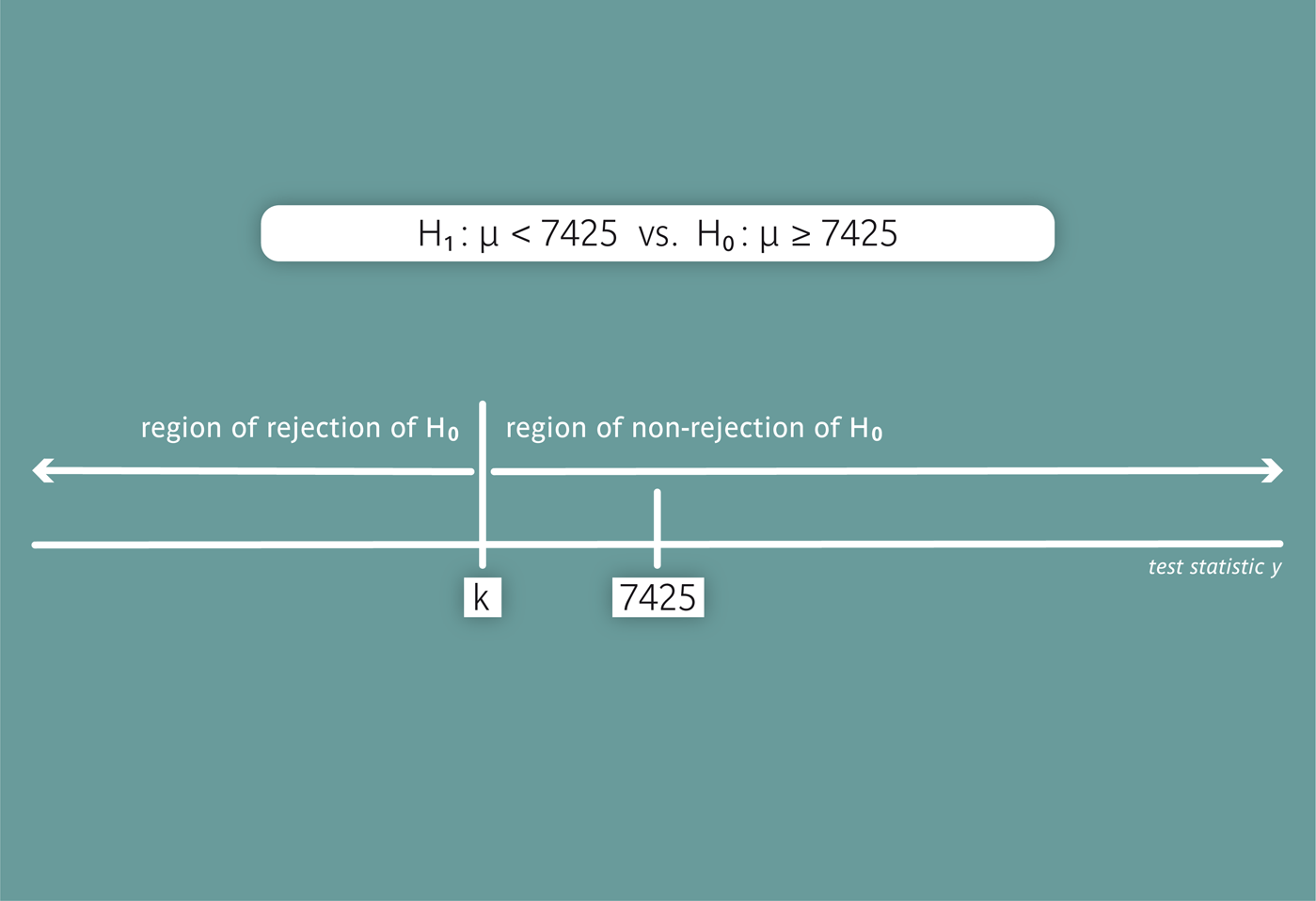
What is obviously missing, is an upper limit \( k \) for observed mean values allowing us to reject \( H_A \). We will first consider such a limit \( k \) as given (but we will soon see how to determine \( k \)). We then decide in favour of \( H_A \) and thus reject the null hypothesis \( H_0 \), if the observed mean value is smaller than \( k \). If the observed mean value is \( \geq k \), we cannot reject \( H_0 \). The non-rejection and the rejection region of \( H_0 \) for this procedure are illustrated in the following figure.
|
Definition 9.1.3
The rejection region of \( H_0 \) includes those values of the test statistic for which we reject \( H_0 \). |
In a more general way, we can describe statistical hypothesis testing as a procedure which enables deciding whether or not to reject \( H_0 \), resp. whether or not to decide in favour of \( H_A \), based on the data of a random sample. Most statistical hypothesis tests are conducted with the help of a test statistic. Such a test statistic can be based on the mean, the median or another measure of the sample. The test consists in making a decision in favour or against the alternative hypothesis, based on the value of the test statistic. To do so, we divide the range of possible values of the test statistic into a rejection and a non-rejection region for \( H_0 \) and reject \( H_0 \) (i.e., decide in favour of \(H_A\)), if our test statistic lies in the rejection region.
|
Synopsis 9.1.3
In a third step we either decide in favour of \( H_A \) and to reject \( H_0 \), if the value of the test statistic lies in the rejection region of \( H_0 \), or not to reject \( H_0 \), if the value of the test statistic does not lie in the rejection region of \( H_0 \). |
As we have learnt in the previous section, we can decide whether or not the null hypothesis \( H_0 \) is compatible with the data at hand, based on a statistical hypothesis test. Table 9.1 illustrates the possible situations which we can encounter in such a decision.
| Decision | Reality | ||||
|---|---|---|---|---|---|
| \( H_0 \) true | \( H_A \) true | ||||
| non-rejection of \( H_0 \) | correct decision | false decision (type II error) | |||
| rejection of \( H_0 \) | false decision (type I error) | correct decision | |||
The table shows that we can make two false decisions, which are referred to as "type I error" and "type II error". In Table 9.2., the decision procedure of a statistical test is compared with a medical diagnostic test. If the disease in question is abbreviated by \(D\), the situation "patient does not have \(D\)" takes the role of \( H_0 \), while the situation "patient has \(D\)" takes the role of \( H_A \). In this case we can also make two false decisions, i.e., by wrongly diagnosing a person with \(D\) as being free of \(D\) based on a false negative test \( \sim \) type II error) or a patient without \(D\) as having \(D\) based on a false positive test \( \sim \) type I error).
| Test result | State of patient | |||
|---|---|---|---|---|
| without disease \(D\) | with disease \(D\) | |||
| negative | correct decision | false decision (false negative) | ||
| positive | false decision (false positive) | correct decision | ||
We will now first take a closer look at type I errors.
The accepted probability for the occurrence of a type I error is denoted by \( \alpha \). It defines the so-called "significance level" of the test and it is usually fixed at \( \alpha = 0.05 \). Therefore the probability that \( H_0 \) is wrongly rejected in favour of the alternative hypothesis must not be larger than \( 0.05 \) ( or \( 5\% \)).
|
Definition 9.1.4
The rejection of a correct null hypothesis in favour of an incorrect alternative hypothesis is referred to as "type I error". The probability of such an error is called "\( \alpha \)-error probability". |
|
Definition 9.1.5
The significance level of a statistical test is the accepted probability for a type I error. |
|
Synopsis 9.1.4
If the null hypothesis is correct and if it is tested at the significance level \( \alpha \), then it is wrongly rejected with a probability of at most \( \alpha \). |
We take up the example of the mean daily calorie consumption \( \mu \) of women between 20 and 30 years of age before their menstruation. We are now interested in the hypothesis \( H_0 : \mu \geq 7425 \) against the hypothesis \( H_A : \mu \lt 7425 \). For this testing problem, we will examine 1000 random samples of 11 women each, in which the individual daily energy uptakes are assumed to be normally distributed with a mean value of \( 7425 \text{ kJ} \) and a standard deviation of \( 1142 \text{ kJ} \). As a test statistic we will use the sample mean value of the 11 measurements. The rejection region of \(H_0\) is of the form \( [-\infty, k )\). With the applet "Type I error", we can determine the value of \( k \) for which \( \alpha \) equals \( 0.05 \).
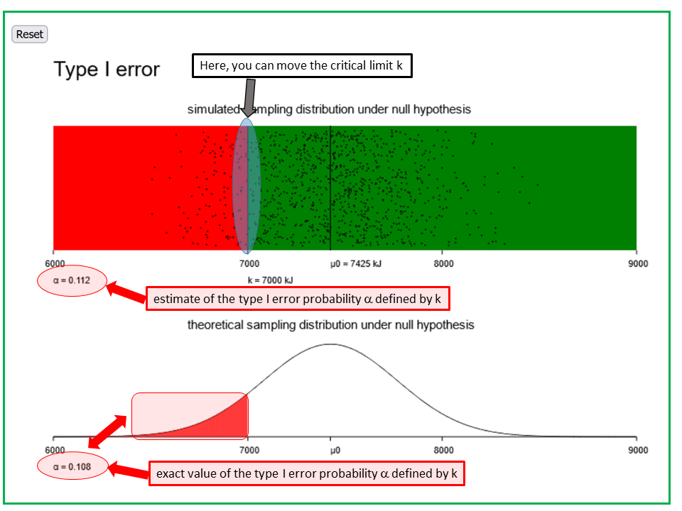
The applet "type-I-error" illustrates the type I-error of a simple statistical test, using the example of daily energy consumption of women before their menstruation. Both panels illustrate the distribution of the means of energy uptake of 11 randomly selected women before their menstruation under the null hypothesis, which states that the true average daily energy uptake in this sub-population of women is no different from the corresponding mean value of 7425 kJ among women in general. The additional assumptions used are that the daily energy uptakes of women before their menstruation follow a normal distribution and that the standard deviation of this distribution equals 1142 kJ.
In the first panel, 1000 mean values of samples of size n=11 were randomly simulated under the above assumptions. Each of these mean values is represented by a dot. In the second panel, the Gaussian bell curve representing the sampling distribution of the means under the concrete null hypothesis that μ0 equals 7425 kJ is displayed. It is calculated under the same assumptions.
The vertical line k represents the critical limit of the test. For observed mean values < k, the null hypothesis is rejected (red area), while it must not be rejected for values > k (green area). The value of k is defined by the pre-specified significance level α of the test. The significance level is the accepted probability of committing an α-error (i.e., of wrongly rejecting the null hypothesis).
The task consists in first defining the significance level α and then to find the corresponding value of k. The value of α displayed in the lower left corner of the upper panel equals the proportion of dots < k (i.e., in the red area). This is an estimate of the probability α of observing a mean value < k under the null hypothesis (and thus of wrongly rejecting the null hypothesis). The exact value of α is provided underneath the lower panel. If is computed under the initial assumptions.
Until now, the alternative hypothesis was formulated in a very general way. However, the probability of a type II error can only be computed, if we postulate a specific value \( \mu \) within \( H_A \). Such a specific alternative hypothesis, which we will denote by \( H_1 \), is called "working hypothesis".
A type II error occurs, if \( H_A \) is correct but our test statistic lies in the non-rejection region of \( H_0 \). The probability of a type II error is denoted by\( \beta \). If we worked with a critical limit \( k = 6500 \text{ kJ} \) in our example of the calorie consumption, then the observed value \( 6753.6 \text{ kJ} \) would lie in the non-rejection region of \( H_0 \).
Let us now assume that the true mean value of daily energy uptake in our sub-population of women equals \( \mu = 7100 \text{ kJ} \) (working hypothesis). Then \( H_A : \mu \lt 7425 \text{ kJ} \) is correct and we wrongly do not reject the null hypothesis \( H_0 \), i.e. we commit a type II error.
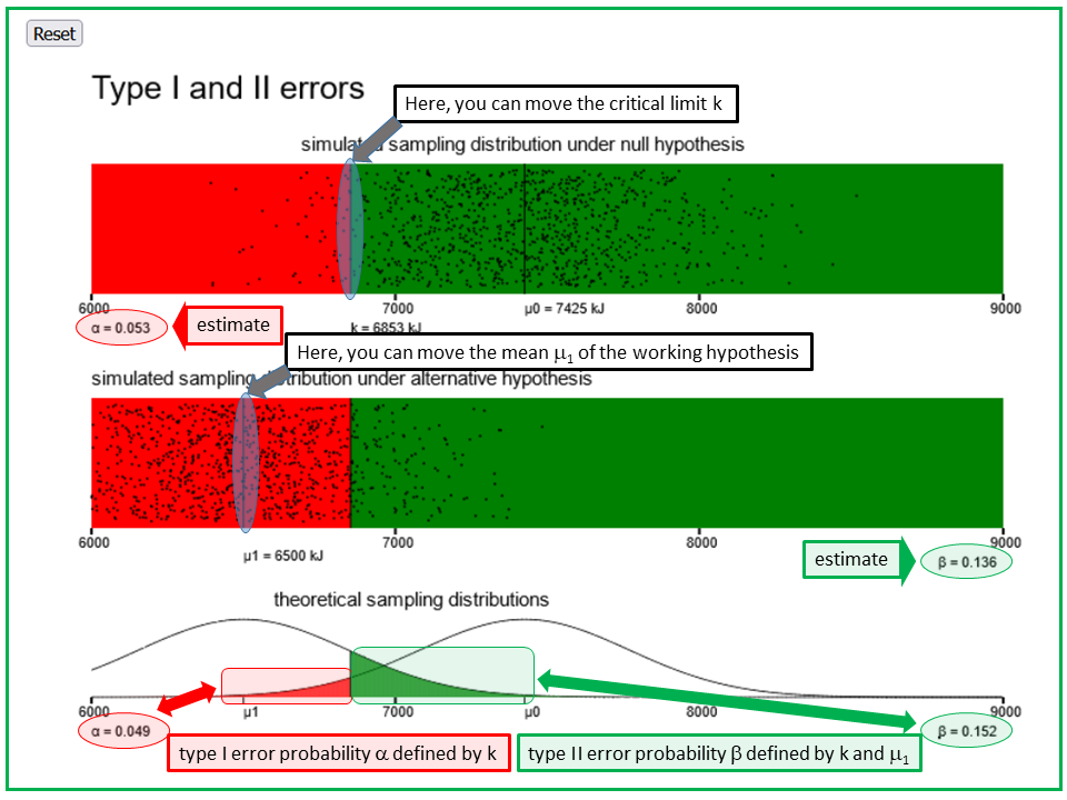
The applet "type-I- and II-errors" illustrates the type I- and the type II-error using the example of daily energy consumption of women before their menstruation. A fixed null hypothesis (i.e., that the true average energy uptake among women before their menstruation, μ0, equals 7425 kJ) is contrasted with a specific alternative hypothesis (working hypothesis) that the true mean value equals μ1. This value can be changed (second panel). The additional assumptions made are that the daily energy uptakes of women before their menstruation follow a normal distribution with a standard deviation of of 1142 kJ.
In the first panel, 1000 mean values of samples of size n=11, each being represented by a dot, were randomly simulated under the null hypothesis and the additional assumptions made. The proportion α of dots > k is indicated in small letters below the lower left corner of the panel. It is an estimate of the probability of the type I- or α-error probability, i.e., of wrongly rejecting the null hypothesis in case it is true. In the third panel (to the right), the Gaussian bell curve representing the true sampling distribution of the means under the additional assumptions and under the null hypothesis (μ0 = 7425 kJ) is displayed. The red area represents the exact value of the α-error probability under the given assumptions.
In the second panel, 1000 means of energy uptake are simulated under a concrete working hypothesis, which differs from the null hypothesis only in the hypothesized mean value, denoted by μ1. The value μ1 can be changed by moving the corresponding vertical line. While moving this line, the 1000 points are constantly updated. The proportion β of dots > k is indicated in small letters below the lower right corner of the panel. This is an estimate of the probability of the type II- or β-error probability, i.e., of wrongly not rejecting the null hypothesis if the working hypothesis is true. In the third panel (to the left), the the Gaussian bell curve representing the true sampling distribution of the means under the additional assumptions and under the specific working hypothesis is displayed. The green area represents the exact value of the β-error probability under the given assumptions.
If you move the vertical line k in the first panel, both the α- and the β-error probability will change.
|
Definition 9.1.6
Failing to reject the null hypothesis if the alternative hypothesis is correct, is referred to as type II error. The probability of committing a type II error is called \( \beta \)-error probability. |
Another important value in a statistical testing problem is the so-called "statistical power". The statistical power of a test with a given significance level \( \alpha \) is the probability of rejecting the null hypothesis \( H_0 \) if the working hypothesis \( H_1 \) is correct. The statistical power of a hypothesis test is closely linked to the \( \beta \)-error probability since the following applies: \[ \text{statistical power} = 1 - \beta \] .
Now work through the applet "Type I and type II errors, n variable" in order to examine the relation between the statistical power and the sample size.
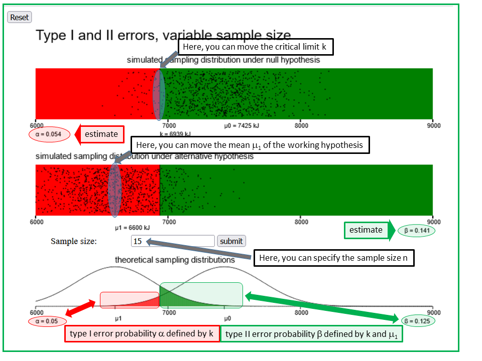
The applet "type-I- and II-errors, sample size variable" illustrates the type I- and the type II-error of a simple statistical test, using the example of daily energy consumption of women before their menstruation. This applet extends the previous one by additionally offering the possibility of specifying the sample size (entry field underneath the second panel).
By default, a sample size of n = 11 is used, corresponding to the size of the observed sample of women. However, you can specify a different value of n. This will change the spread of the points and of the bell curves. If you choose n > 11, the spread will decrease, if you choose n < 11, it will increase.
After having pre-specified μ1 (i.e., the working hypothesis), α (= 0.05, in general) and the accepted value β of the probability of a type II error (e.g., 0.2 or 0.1), you can try to find the sample size which is needed for α and β to reach the pre-specified values.
Hint: If you change n, then you must adjust k to get α = 0.05 again. By monitoring β you will see in which direction the value of n must be changed to get closer to the pre-specified value of β.
|
Definition 9.1.7
The probability of being able to reject the null hypothesis, under the assumption that \( H_1 \) is correct, is referred to as statistical) power. |
Notice that the power depends on the significance level chosen.
|
Synopsis 9.1.5
The following relation holds between the power of a statistical hypothesis test and the probability \( \beta \) of a type II error: power = \( 1 - \beta \) . |
We can also illustrate the probabilities of the different test decisions in a two by two table (Table 9.3). As in tables 9.1 and 9.2, we will again compare the respective decision probabilities with those of a diagnostic test. Again, we let \( H_0 \) correspond to the situation of a "patient without the disease \(D\)" and \( H_A \) to the situation of a "patient with the disease \(D\)".
| \( H_0 \) = true | \( H_A \) = true | |||
|---|---|---|---|---|
| Probability of not rejecting \( H_0 \) | \( 1 - \alpha \) | \( \beta \) | ||
| Probability of rejecting \( H_0 \) | \( \alpha \) (= significance level) |
\( 1 - \beta \) (= power) |
||
| without disease | with disease | |||
| probability of negative test result | specificity | 1 - sensitivity | ||
| Probability of positive test result | 1-specificity | sensitivity | ||
In the following figure, the sampling distributions of the mean values of the calorie consumption of \(n\) women before their menstruation are illustrated under \( H_0 \) (right density curve with the centre \( \mu_0 \)) and under \( H_1 \) (left density curve with the centre \( \mu_1 \)).
We know from chapter 8 that the spread of the sampling distribution of a mean value is described by the standard error which depends on the following two factors:
|
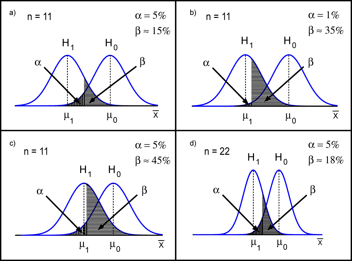
Synopsis 9.1.6
The following factors influence the probability \( \beta \) of a type II error and thus the power \( 1 - \beta \) of a statistical hypothesis test (provided that \(H_1 \neq H_0\)): a) The smaller the significance level \( \alpha \) (accepted probability of a type I error), the bigger \( \beta \) and thus the smaller the power \( 1 - \beta \) (for a fixed sample size \( n \)). b) The smaller the difference between \( H_0 \) and \( H_1 \), the bigger \( \beta \) and thus the smaller the power \( 1 - \beta \) (for a fixed sample size \( n \). c) The bigger the sample size \( n \), the smaller \( \beta \) and thus the bigger the power \( 1 - \beta \). d) The smaller the standard deviation \( \sigma \) of the variable, the smaller \( \beta \) and thus the bigger the power \( 1 - \beta \) (for a fixed sample size \( n \)). |
The measurements of the 11 women provided a mean value of \( 6753.6 \text{ kJ} \). We are now interested in the probability of observing an even smaller mean value in a new random sample of equal size from a population with \( \mu = 7425 \text{ kJ} \) and \( \sigma = 1142 \text{ kJ} \) (thus corresponding to \( H_0 \)). This probability is referred to as "\( p \)-value" of the observed mean value. Use the applet "p-value" to find the approximate \( p \)-value of the observed mean value of \( 6753.6 \text{ kJ} \).
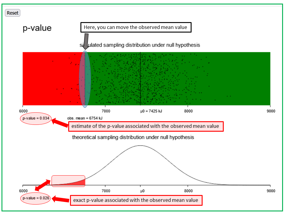
The applet "p-value" illustrates the p-value of a simple statistical test, using the example of daily energy consumption of women before their menstruation. It is almonst a copy of the applet "Type I-error", the only difference being that "k" is replaced by "observed mean". Both panels illustrate the distribution of the means of energy uptake of 11 randomly selected women before their menstruation under the null hypothesis that the true average daily energy uptake in this subgroup equals the mean value of 7425 kJ among women in general.
In the upper panel, 1000 such mean values, each being represented by a dot, were randomly simulated under the assumption that the values of energy uptake of pre-menstrual women follow a normal distribution with a mean value of 7425 kJ and a standard deviation of 1142 kJ. In the lower panel the theoretical distribution of the sample means is represented by a Gaussian bell curve.
To decide whether the observed mean value of 6754 kJ is "realistic" under the null hypothesis, you can move the vertical line "observed mean" to this value and see what the proportion p of dots < k is. This value is indicated in small letters below the lower left corner of the panel. In both panels, the area to the left of "observed mean" appears in red color and the area to the right in green color. While value of p below the upper panel is an estimate, the one below the lower panel is exact under the assumptions made.
The value p equals the probability, computed under the null hypothesis, of observing in a next random sample of 11 women before the menstruation a mean value of energy uptake which is (even) lower than the one observed.
if the p-value is smaller than the pre-specificed significance level α, then the observed result is statistically significant at this level and the null-hypothesis can be rejected.
The \( p \)-value can be defined in a more general way as follows:
|
Definition 9.1.8
First we calculate the value \( t \) of an appropriate test statistic from the data of the observed sample. Then, conditional on the null hypothesis \( H_0 \) being true, we determine the probability that a new random sample of the same size from the same population would provide a test statistic at least as unlikely (under \( H_0 \) as \(t\) (i.e., arguing against \( H_0 \) at least as strongly as \( t \)). |
This phrasing is tuned to small \( p \)-values. For large \( p \)-values we would rather speak of values of the test statistic which argue even less for \( H_1 \) than \( t \). A small \( p \)-value means that the probability of getting a value of the test statistic at least as "extreme" as the observed one, under the null hypothesis, is small. Accordingly, the observed value of the test statistic would then be an "extreme" value itself if the null hypothesis were true. A small \( p \)-value therefore argues against the plausibility of the null hypothesis. The following rule applies:
|
Synopsis 9.1.7
If the \( p \)-value is smaller than \( \alpha \), then we can reject \( H_0 \) at the significance level \( \alpha \) and decide in favour of the alternative hypothesis. |
Important concluding remark: "Statistical significance" must not be confounded with "relevance". In small studies, even relevant differences may fail to translate into statistically significant results, due to a lack of statistical power. On the other hand, irrelevant differences may become statistically significant in large studies, due to excessive statistical power. Therefore, an important goal of study design is to choose the sample size(s) such that the statistical power of observing a statistically significant result will be high, in case of a relevant difference between \( H_1 \) and \( H_0 \).
A statistical hypothesis test starts with the formulation of a hypothesis \( H_A \) postulating a certain difference between two populations, a treatment effect or an existing relation between two variables. The null hypothesis, denoted by \( H_0 \), denies the existence of such a difference, treatment effect or relation. As probability calculations are primarily based on the null hypothesis, the hypothesis \( H_A \) is also called "alternative hypothesis". In order to decide whether to reject \(H_0\) (and thus to favour \( H_A \)) or not, we use a test statistic which can be calculated from one or multiple samples. The range of values of the test statistic is divided into two intervals: the rejection and the non-rejection region of \( H_0 \). The decision rule is as follows:
The accepted probability of a type I error is referred to as "significance level" of the test and is denoted by \( \alpha \). This value is fixed before carrying out the test. Common values are \( 0.05 \) and \( 0.01 \). With \( \alpha = 0.05 \), one accepts a type I error to occur in \( 5\% \) of cases where \(H_0\) is true. The probability of a type II error under a specific working hypothesis \( H_ 1 \) is denoted by \( \beta \). Therefore, the power of a test, i.e. the probability of being able to reject \( H_0 \) if the working hypothesis \( H_1 \) is correct, equals \( 1 - \beta \).
If the significance level is fixed, the power increases and \( \beta \) decreases with increasing sample size. The "\( p \)-value" is the probability of observing a value of the test statistic which would be at least as unlikely as the observed value under the null hypothesis. If we work with the \( p \)-value, the following decision rule applies:
In the first case. we say that the observed result is "statistically significant" (at the level \( \alpha \)). In the second case, the result is said to be "(statistically) non-significant". With a non-significant result, we have to consider the possibility that an observed difference has been caused by chance alone.
"Statistical significance" must not be confounded with "relevance". It must be kept in mind that the \( p \)-value strongly depends on the size of the study. The same observed difference or effect may have a large p-value in a small study and a small p-value in a large study.