
|
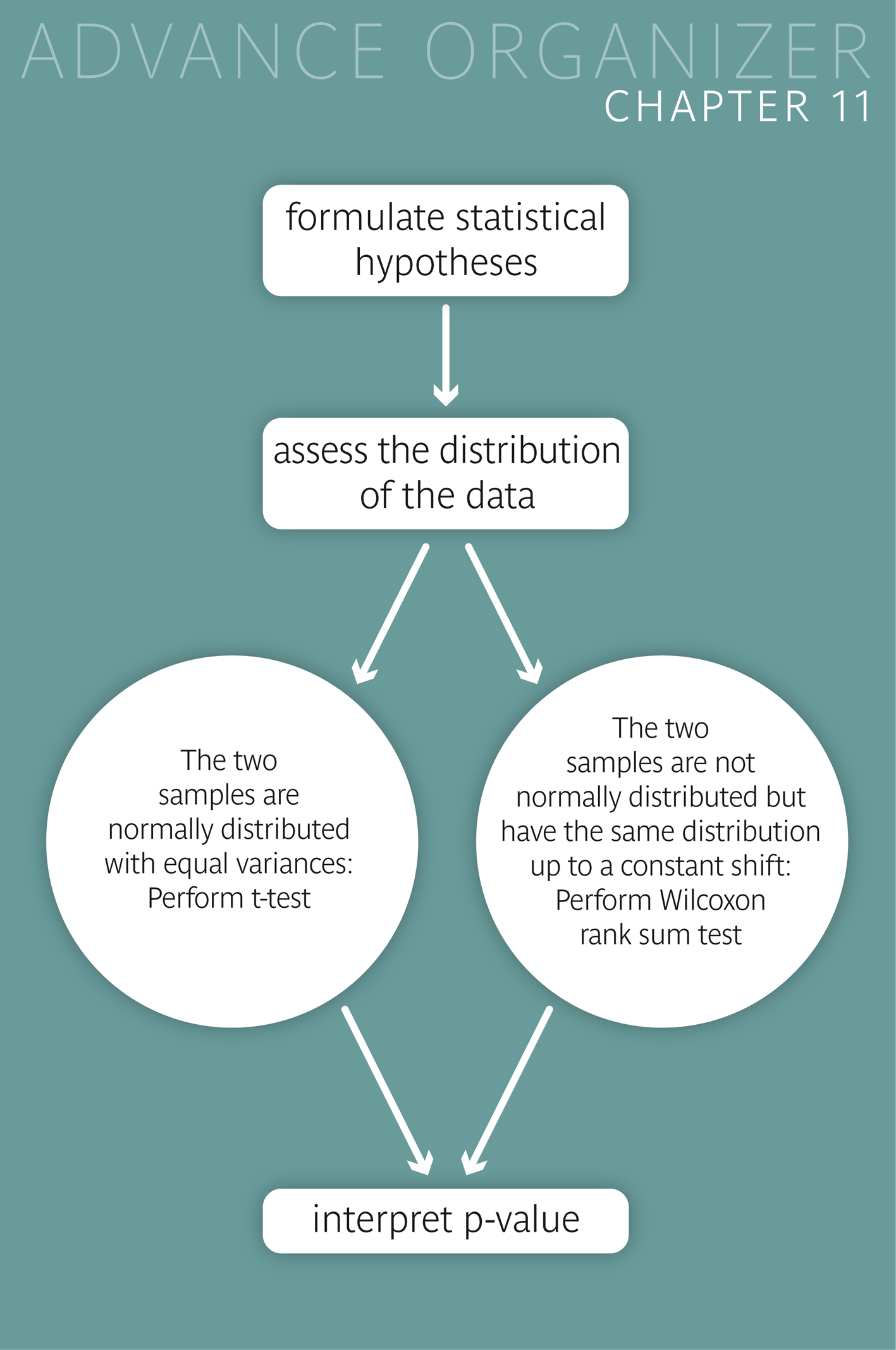
Often, in clinical studies, two different treatments are tested in separate groups of patients. In epidemiological studies, two different sub-populations are often compared with regard to a specific variable. If this is a quantitative variable and we want to find out if its mean value differs significantly between the two observed groups, the following tests can be used: For normally distributed data the two-sample \(t\)-test is used. Otherwise the nonparametrical Wilcoxon rank sum test (also called the Mann-Whitney- U-test) provides an alternative. |
|
Educational objectives
After having worked through this chapter you will be familiar with the tests which are used to evaluate differences in the location of two independent samples with respect to a quantitative variable. You will also know the conditions for the validity of these tests, and you will be able to decide which tests to apply in concrete situations. You will be able to classify statistical testing situations based on a given set of criteria. Key words: Two-sample \(t\)-test, Wilcoxon rank sum test or Mann-Whitney-U-test, independent samples.Previous knowledge: mean value, median (chap. 3), normal distribution (chap. 6), statistical hypotheses, statistical hypothesis testing, significance level, p-value (chap. 9) Central questions: Which test should be used to evaluate the difference in the location of two independent samples with respect to a quantitative variable? |
So far, we have examined situations which could be translated into settings with just one sample (situations with one single sample or with two paired samples). In this chapter we will treat situations with two independent samples. We again start with an example:
Several theories concerning the development of schizophrenia imply changes in the activity of the hormone dopamine in the central nervous system. In a study by Sternberg et al. (1982) [1], \(25\) hospitalised schizophrenia patients were treated with an antipsychotic drug and classified as psychotic (\(10\) patients) or non-psychotic (\(15\) patients) after the treatment. Furthermore the dopamine activity in the liquor (cerebro-spinal fluid) was determined for every patient.
Additionally the ratio between the level of the dopamine beta hydroxylase (DBH) and the protein concentration was determined. For the group of the psychotic patients this ratio reached a mean of \(0.0243\) resp. \(2.43\%\) and for the group of non-psychotic patients a mean of \(0.0164\) resp. \(1.64\%\). The question arises if the mean DBH-concentration of psychotic patients (\( = \mu_P \) ) differs from the one of non-psychotic patients (\(= \mu_N\) ). This means that we are interested in the alternative hypothesis \[ H_A : \mu_P \neq \mu_N \,,\] with the corresponding null-hypothesis \[ H_0 : \mu_P = \mu_N \] In the following two sections we will introduce procedures for such testing problems.
Under the two conditions
the test-statistic of the two-sample \(t\)-test for equal variances follows a \(t\)-distribution with \(n_1 + n_2 - 2\) degrees of freedom. we can treat our testing problem with the two-sample \(t\)-test for equal variances (classical \(t\)-test).
In practice, the two conditions can be slightly relaxed, by requiring approaximate normality and similar variances (or standard deviations).
We look at the Q-Q-plot of the data of the schizophrenia example in figure 11.2 and reason that both the measurements of psychotic and non-psychotic patients are approximately normally distributed.
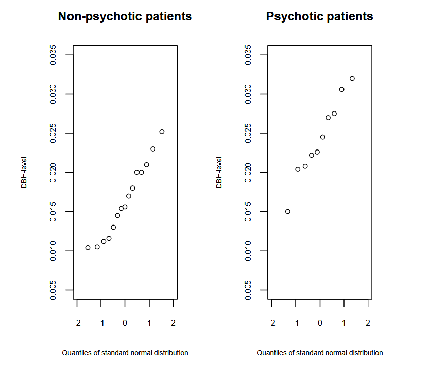
The sample standard deviation of the measurements of the psychotic and non-psychotic patients are \( s = 0.00514 \) and \( s = 0.00470 \), respectively. The ratio of the standard deviations does not deviate much from 1. Therefore we can hypothesize that the standard deviations at the population level are not very different either.
The respective test statistic consists of a standardised difference of the two sample means.
As in the one-sample \(t\)-test, the difference of the mean values is divided by its standard error. The resulting ratio \( t \) has a \(t\)- distribution with \( n_1+n_2-2 \) degrees of freedom under the null hypothesis and the conditions stated above. Here, \(n_1\) and \(n_2\) denote the two sample sizes. The calculation of the standard error, however, is a bit more complicated than in the one-sample \(t\)-test. It is given in section 11.5 for those interested.
We apply the two-sample \(t\)-test to the \(25\) observations and get a \(p\)-value of \( 0.0007 \). Therefore we can reject \( H_0 \) at the significance level \( \alpha = 0.05 \) and decide in favor of the alternative hypothesis that the mean DBH-concentration of the liquor differs between psychotic and non-psychotic patients.
An important characteristic of the two-sample \(t\)-test is that the normality condition can be ignored in large samples. This follows from the approximate normality of the sampling distribution of the mean, which was discussed in chapter 8.
However, the condition of approximately equal standard deviations (or variances) must be fulfilled even with large samples, unless the two sample sizes are equal or similar. Of course, a natural question to ask is how big a large sample must be. There is no general answer to this question.
However, there are common situations in which concrete answers are possible. For instance, in experimental studies, equally sized groups are common. In this case, a group size \(n \geq 40 \) is generally sufficient for the classical two-sample \(t\)-test to be valid [cf.[4], pp 418 ff].
In a study by Evans et al. (1991) (cf. [2], page 231 and [3]) the influence of diabetes on foot-problems was examined. For this study a tendon reflex was examined in \(79\) non-diabetics and \(74\) diabetics who were between \(70\) and \(90\) years old. Measurements were graded with a score (\(1-3\)). The observed mean values and standard deviations are listed in table 11.1.
| Sample | sample size | Mean value | Standard deviation |
|---|---|---|---|
| diabetics | 74 | 2.1 | 1.1 |
| non-diabetics | 79 | 1.6 | 1.2 |
The question arises if the mean reflex of diabetics differs from the one of non-diabetics. The standard deviations are similar in both groups and the sample sizes are both larger than \(25\). Thus, we can use the two-sample \(t\)-test to solve this testing problem. It provides a \(p\)-value of \(0.008\). Thus, the mean tendon reflex score differs significantly between the two groups at the \(5\%\)-level.
|
Synopsis 11.1.1
In the case of two independent samples of quantitative data, the two-sample \(t\)-test can be used to examine the difference in the two sample means if 1) the data are close to normally distributed in both populations and the variances are similar. 2) the sample sizes or the variances are similar and \( n_1+n_2 \geq 40 \). In case of doubt, the \(t\)-test for unequal variances, which is treated in the next section, should be used. This particularly applies to doubts whether the variances may be considered as sufficiently similar or not. |
If the sample sizes are similar, the classical two-sample \(t\)-test is robust against violations of the "equal variance"-condition. However, if both the sample sizes and variances are different, the classical two-sample \(t\)-test becomes invalid.
As an alternative, the two-sample \(t\)-test for unequal variances can be used. It is also known under the name "Welch-test".
In this test, the standard error of the difference of the sample means has a different form (cf. section 11.5).
Unfortunately, the statistic of this test does not follow an exact \(t\)-distribution under the null hypothesis of equal population means. However, if the sample sizes are not too small, the null-distribution of this test-statistic can be well approximated by a \(t\)-distribution with an "adjusted" number of degrees of freedom.
The formula for the computation of this adjusted number is quite complicated. Fortunately, this test is implemented in most statistics programs. Moreover, using the smaller of the two numbers \(n_1-1)\) and \(n_2-1)\) for the degrees of freedom, one obtains a conservative test, i.e., a test with a type I-error probability \(\lt \alpha\).
The authors of [1] recommend using this test rather than the classical two-sample \(t\)-test in case of doubt. They give the following recommedations (cf.[4], pp 418 ff) for the use of this test.
a) If \(n_1+n_2 \leq 15\), then the variable \(X\) should look close to normally distributed in both samples.
b) If \(n_1 + n_2 \geq 40\), the test can even be used if \(X\) has a clearly skewed distribution.
If the \(t\)-test for unequal variances is applied to the two examples of section 11.1.1, the \(p\)-values turn out to be \(0.0011\) and \(0.008\), respectively. Thus, the \(p\)-value slightly increases in the first example, but remains the same in the second one. In both examples, the null-hypothesis of equal population means can again be rejected at a two-sided significance level of \(\alpha = 0.05\).
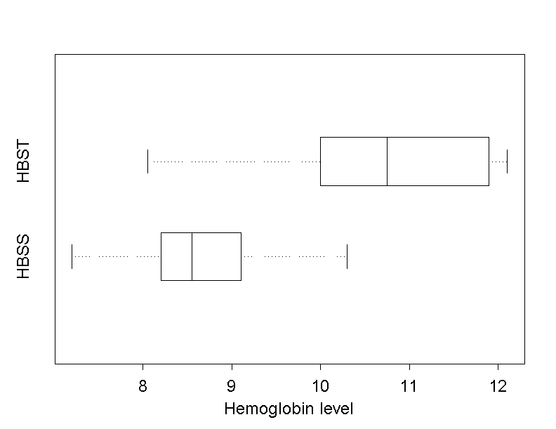
In a study by Anionwu E. et al. (1981) (cf. [5]) it was examined if the type of disease has an influence on the haemoglobin concentration in the blood of patients with sickle cell disease. The haemoglobin concentration was measured (in \(g/dl\)) in \(16\) patients with type HBSS and \(10\) patients with type HBST. The respective measurements are illustrated in a boxplot in figure 11.3
We further take a look at the Q-Q plot of the measured values of both groups in figure 11.4.
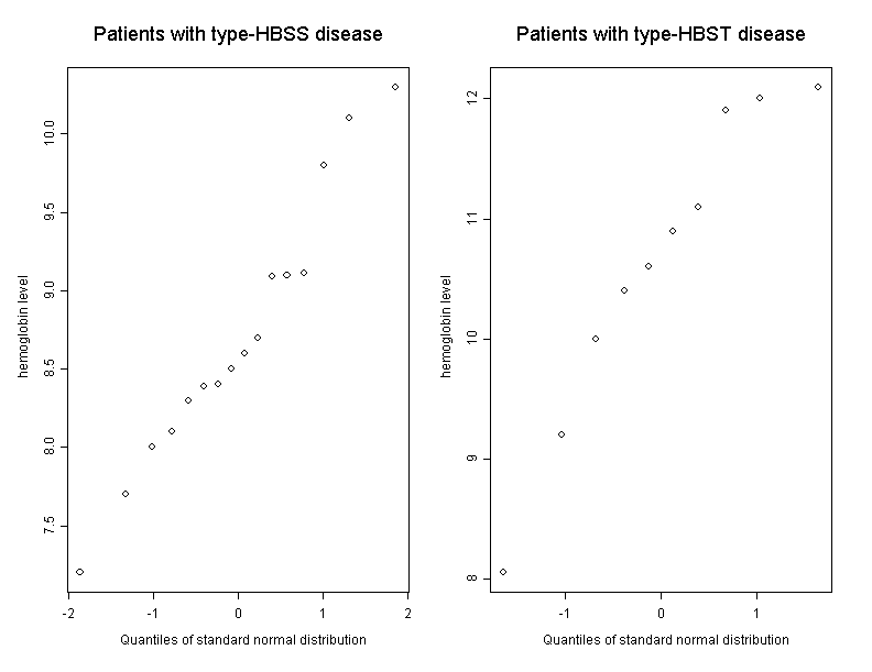
After having examined the graphs we doubt that the data are normally distributed in the underlying populations. Furthermore the sample sizes are small. Therefore the two-sample \(t\)-test is not a valid option for the analysis of these data.
On the other hand we assume that the data of both groups are equally distributed except for their location, even though the illustration in figure 11.3 does not exactly support this. (In the following section we will briefly discuss the consequences of a violation of this condition).
The sample standard deviations are \(0.85\) in the HBSS-group and \(1.29\) in the HBST-group. Since the ratio of the two standard deviations does not deviate too much from 1, we can hypothesize that the population standard deviations are not too different either. Under the condition that the distributions of heamoglobin are identical in both populations up to a shift (i.e., that they are congruent), we can apply the so-called "Wilcoxon rank sum test" to test the null hypothesis \[ H_0 : \mu_{HBSS} = \mu_{HBST} \] against the two-sided alternative hypothesis \[ H_A : \mu_{HBSS} \neq \mu_{HBST} \] where \( \mu_{HBSS} \) denotes the mean haemoglobin concentration in the HBSS-population and \( \mu_{HBST} \) the mean haemoglobin concentration in the HBST-population.
As with the Wilcoxon signed rank test, the test statistic \( W \) of the Wilcoxon rank sum test is based on the ranking of the values and not on the measured values themselves. While the two-sample \(t\)-test is based on the difference in the sample means of the original data, the Wilcoxon rank sum test uses the difference in the means of the corresponding ranks. The rank variables of the haemoglobin data are listed in table 11.2.
| HBSS-group | HBST-group | ||
|---|---|---|---|
| Value | Rank | Value | Rank |
| 7.2 | 1 | ||
| 7.7 | 2 | ||
| 8.0 | 3 | ||
| 8.05 | 4 | ||
| 8.10 | 5 | ||
| 8.30 | 6 | ||
| 8.39 | 7 | ||
| 8.40 | 8 | ||
| 8.50 | 9 | ||
| 8.60 | 10 | ||
| 8.70 | 11 | ||
| 9.09 | 12 | ||
| 9.10 | 13 | ||
| 9.11 | 14 | ||
| 9.20 | 15 | ||
| 9.80 | 16 | ||
| 10.00 | 17 | ||
| 10.1 | 18 | ||
| 10.3 | 19 | ||
| 10.4 | 20 | ||
| 10.6 | 21 | ||
| 10.9 | 22 | ||
| 11.1 | 23 | ||
| 11.9 | 24 | ||
| 12.0 | 25 | ||
| 12.1 | 26 | ||
The mean values of the ranks are \(9.625\) (HBBS-group) and \(19.7\) (HBST- group). They clearly differ from one another.
One can calculate exact \(p\)-values for small sample sizes, but for larger samples, statistics programs calculate the \(p\)-values using an approximation formula.
For our testing problem, the exact \(p\)-value is \(0.0006\). Based on this test result, we reject the null hypothesis and decide in favor of the alternative hypothesis stating that the mean haemoglobin concentration of patients with the disease type HBSS differs from the one of patients with disease type HBST.
If, up to a shift in location, the data have the same distribution in both populations (i.e., if the distributions are congruent), the difference in the mean values is equal to the difference in the medians at the population level. In this case, the Wilcoxon rank sum test will simultaneously test equality of the medians against their difference.
If the two distributions have similar shapes but different spreads, then the Wilcoxon rank sum test rather captures differences in the medians than differences in the means. Hence it can be generally said that the Wilcoxon rank sum test measures differences in the medians rather than differences in the means.
The Wilcoxon rank sum test generally captures differences between two distributions well if their cumulative distribution functions do not intersect each other.
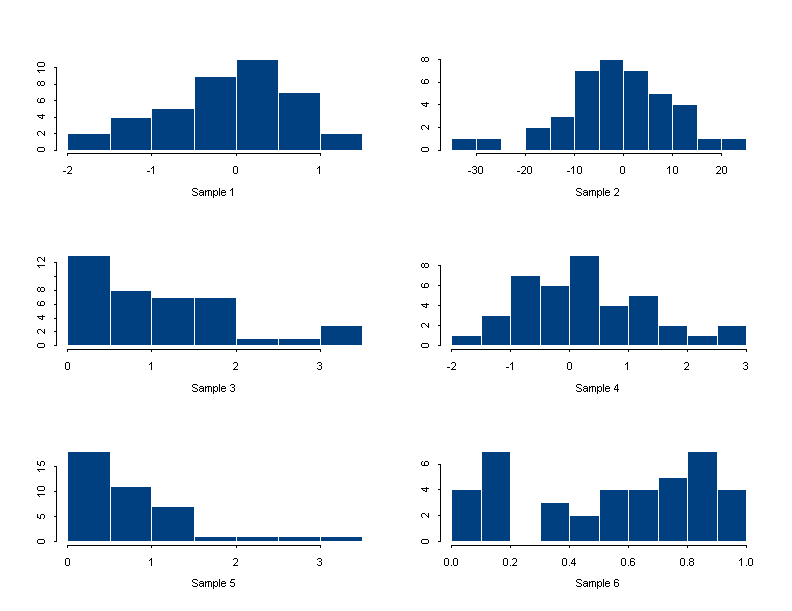
Note: Consider the scaling of the x-axis in each case.
|
Synopsis 11.2.1
Assume that a quantitative variable \( X \) has been observed in two independent random samples from different populations.
|
Recall that empirical distributions can be very well compared using boxplots. Case 1) corresponds to a situation where the two boxplot are essentially congruent, while case 2) corresponds to a situation where the boxplots have a similar shape but a different length.
Maths enthusiasts can gain an insight into the functionality of this test with the applet "Wilcoxon rank sum test".
![]()
The applet "Rank sum test" illustrates the working of the Wilcoxon rank sum test. After pressing the key "New Experiment", five blue and five red balls drop down from the ceiling and jump back from the floor, each one to a different height. There are two alternative random mechanism producing the jumping heights of the balls. The first one follows the null hypothesis that the average jumping heights of the red and the blue balls are identical, while the other mechanism follows a specific alternative hypothesis that the mean jumping height of the blue balls is higher than the one of the red balls. When starting the experiment, each of the two hypotheses has the same probability of being selected. You are asked to decide whether the null hypothesis or the alternative hypothesis was selected and to press the respective key at the bottom. The ranks of the jumping heights of the blue and red balls are displayed in the stick diagram to the right, the sums of the ranks of the red and the blue balls are indicated underneath the stick diagram, and the difference D between the sum of ranks of the blue and the red balls is displayed in the diagram below the balls as a vertical green line. The black vertical line at 0 represents the mean of D under the mull hypothesis. Thus, a large positive difference speaks in favour of the alternative hypothesis, while a value of D close to 0 rather speaks in favour of the null hypothesis.
If you press the key "Random coloring", the red and the blue colors are re-distributed randomly across the 10 balls, the stick diagram to the right is updated and the difference D is re-computed and represented as dot in the diagram below the balls. By pressing the key repeatedly, you can observe the dots which appear to the right of the green line. Theit proportion among all dots is an estimate of the one-sided p-value of the initial value of D. It is indicated underneath the diagram. By pressing the key "100 random colorings", 100 new dots are generated.
Figure 11.6 gives an overview of the different testing situations and the criteria which have to be considered in the choice of a statistical test. Some of these situations were treated in the present chapter and in chapter 10. Others will be treated in chapter 12.
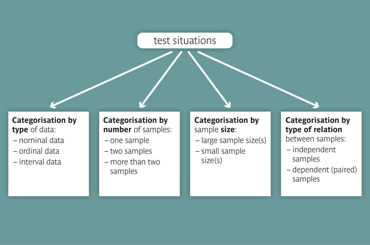
The primary criterion for categorizing testing situations is the type of data compared
In a second step the testing situations are distinguished based on the number, dependency and size of the samples to be compared. These different situations ask for different test procedure. We differentiate between
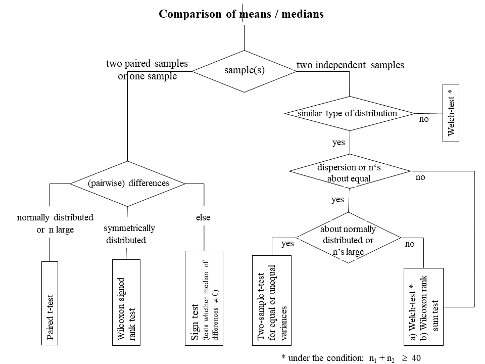
The following flow chart provides an overview of the testing situations with quantitative variables observed in one sample, two paired samples or two independent samples
|
Synopsis 11.3.1
A testing situation can be characterised based on the following criteria: a) the data type b) the number of samples c) the dependency structure of the sample(s) d) the sample size(s). |
We have the following three options to test if the difference in the means of a variable \( X \) from two random samples is statistically significant:
The two-sample \(t\)-test for equal variances can be applied in most situations, if
The two-sample \(t\)-test for unequal variances can be applied in most situations, as long as the sum of the two sample sizes exceeds 40.
Alternatively, the Wilcoxon rank sum test can be used, if, up to a shift in location, the distributions of \(X\) look almost the same in the two samples.
If the distribution of \(X\) has a similar shape but a different spread in the two samples, the Wilcoxon rank sum test captures differences between the medians rather than between the means.
In general, a testing situation can be classified according to the criteria "data type", "number of samples", "sample size" and "dependency structure of the samples".
Assume that a variable \( X \) is normally distributed in two populations with mean values of \( \mu_1 \) and \( \mu_2 \) and standard deviations \( \sigma_1 \) and \( \sigma_2 \), and that we have two independent random sample of size \( n_1 \) and \( n_2 \) from these populations. Then the standard error of the difference \( \bar{x}_2 - \bar{x}_1 \) equals \( \sqrt{\frac{\sigma_1^2}{n_1}+\frac{\sigma_2^2}{n_2}} \). It can be estimated by \[ SE_1 = \sqrt{ \frac{s_1^2}{n_1}+\frac{s_2^2}{n_2} } \,, \] where \( s_1 \) and \( s_2 \) are the standard deviations of \( X \) in the two samples.
This is the estimate of the standard error of \( \bar{x}_2 - \bar{x}_1 \) in the two-sample \(t\)-test for unequal variances.
However, if \( \sigma_1 = \sigma_2 \), a better estimate is \[ SE_2 = \sqrt{\frac{1}{n_1}+\frac{1}{n_2}} \times \sqrt{ \frac{ (n_1-1)\times s_1^2 + (n_2-1)\times s_2^2}{n_1 + n_2 - 2}} \,.\] This is the estimate of the standard error of \( \bar{x}_2 - \bar{x}_1 \) in the two-sample \(t\)-test for equal variances.
Under the condition that
For large sample sizes, the ratio \[ t = \frac{\bar{x}_2 - \bar{x}_1}{SE_1} \] approximately follows a standard normal distribution under the null hypothesis that \( \mu_2 = \mu_1 \), even if \( \sigma_2 \) and \( \sigma_1 \) or \( n_1 \) and \( n_2 \) are clearly different, provided that the distribution of \( X \) is not too skewed. Thus, in this case the critical limits for the observed \(t\)-statistic can be set to \(-1.96\) and \(1.96\).
[1] D.E. Sternberg, D.P. VanKammen, P. Lerner, W.E. Bunney (1982)
Schizophrenia: dopamine beta-hydroxylase activity and treatment response.
Science 216 (6), pp 1423-5, DOI: 10.1126/science.6124036
Data copied from page 37 of
D.J. Hand, F. Daly, A.D. Lunn, K.J. McConway and E. Ostrowski
A Hndbook of Small Data Sets
Chapman and Hall, London, 1994
[2] W.W. Daniel, (1995)
Biostatistics
John Wiley and Sons Inc.
[3] S.L. Evans, B.P. Nixon, I. Lee, D. Yee, A.D. Mooradian (1991)
The prevalence and nature of podiatric problems in elderly diabetic patients
J Am Geriatr Soc 39 (3), pp 241-5, DOI: 10.1111/j.1532-5415.1991.tb01644.x
[4] D.S. Moore, G.P. McCabe, (1993)
Introduction to the practice of statistics
W.H. Freeman and Company, New York
[5] E. Anionwu, D. Watford, M. Brozovic, B. Kirkwood (1981)
Sickle cell disease in a British urban community
British Medical Journal (Clin Res Ed) 282, pp 283-6, doi: 10.1136/bmj.282.6260.283.
Data copied from page 247 of
D.J. Hand, F. Daly, A.D. Lunn, K.J. McConway and E. Ostrowski
A Handbook of Small Data Sets
Chapman and Hall, London, 1994
[6] D.G. Altman, (1994)
Practical Statistics for Medical Research
Chapman and Hall, London.