
|
Does the mean of a specific variable \(X\) in a certain group of people differ from the respective mean in a "reference population"? On average, do the values of a blood parameter change during a medical treatment? Such questions can be answered with the testing procedures treated in this chapter. The "one-sample t-test" and the "Wilcoxon signed rank test" are ideal for such comparisons. The correct interpretation of the results of these tests is important. Analogous questions regarding the median of a variable \( X \) rather than its mean can be addressed using the "sign test". |
|
Educational objectives
After having worked through this chapter you will be able to choose the adequate testing procedure in a concrete situation with a quantitative variable having been observed in a random sample, if a hypothesis about the mean or the median of the variable at the population level has been formulated. Moreover, you can justify your decision, and you can correctly interpret the resulta of the respective tests. Key words: one-sample t-test, Wilcoxon signed rank test, sign test, paired samples, one-sided and two-sided hypotheses. Previous knowledge: sample statistics (chap. 3), population parameters (chap. 4), normal distribution, Q-Q-plot (chap. 6), standard error, confidence interval (chap. 8), statistical hypotheses, statistical hypothesis testing, significance level, p-value (chap. 9) Central questions: Which tests are suitable for comparing the mean or the median of a variable in a random sample from a specific sub-population with a reference value? How can this question be translated into the language of statistics? Which criteria have to be considered when applying these tests? |
The methods introduced in this chapter are ideal for comparing the mean of a variable in a random sample with a reference value. Let us have a look at some examples.
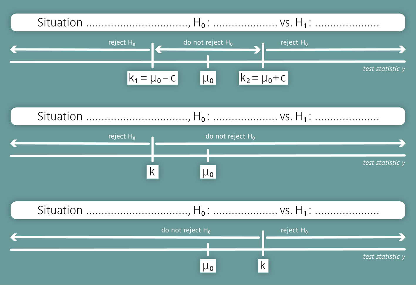
Situation 1: In a former study it was claimed that the mean age \( \mu \) of a certain patient population equals \( \mu_0 = 20.7 \,\text{years} \). Since we are suspicious about this value, we draw our own sample with \( n \) measured values \( x_1, . . . , x_n \) and test the null hypothesis \[ H_0 : \mu = \mu_0 = 20.7 \] against the two-sided alternative hypothesis \[ H_A : \mu \neq 20.7 \,\, \text{(the mean is different from 20.7 years)}, \] at a prespecified significance level \( \alpha \). If we can reject \( H_0 \), our suspicion is confirmed. Otherwise, we may have to revisit our objections against the value \( \mu_0 \). This is an example of a two-sided test, as \( H_A \) includes values of \( \mu \) on both sides of \( H_0 \).
Situation 2: The study of the calorie consumption aimed to show that the mean daily calorie consumption \( \mu \) among women before their menstruation wass smaller than \( \mu_0 = 7425 \,\text{kJJ} \). This leads to the null hypothesis \[ H_0 : \mu \geq \mu_0 = 7425 \] against the one-sided alternative hypothesis \[ H_A : \mu \lt \mu_0 = 7425 .\] We thus test the alternative hypothesis, that the mean calorie consumption is smaller than \( 7425 \,\text{kJ} \). This is an example of a one-sided test with \(H_A \lt H_0\).
Situation 3: In a study, it was claimed that the mean monthly number of visits by relatives of chronic patients in a nursing home is at most \( \mu_0 = 5 \). We have doubts about this and therefore record the number of visits in a random sample of \( n \) patients during one year to test the following hypothesis \[ H_0 : \mu \leq \mu_0 = 5 \] against the one-sided alternative hypothesis \[ H_A : \mu \gt \mu_0 = 5 .\] This is an example of a one-sided test with \(H_0 \lt H_A\).
Tests with a two-sided alternative hypothesis are simply called "two-sided test", while tests with a one-sided alternative hypothesis are referred to as "one-sided tests".
In figure 10.2, the specific non-rejection and rejection regions of the three situations are illustrated schematically, but parts of the labels are missing. Try to complete them!
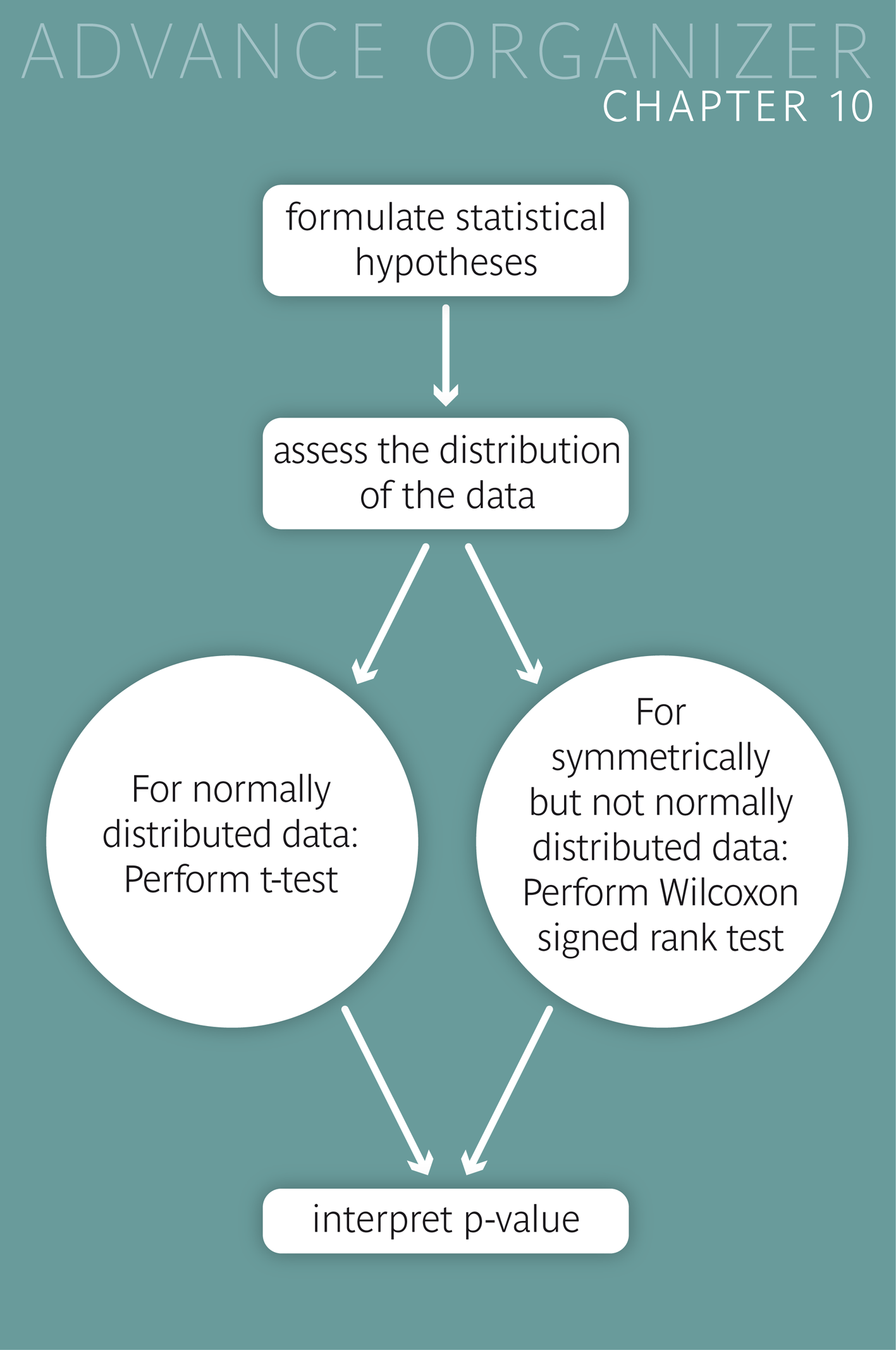
In the following we will consider two testing procedures, which are suitable to address the testing problems introduced.
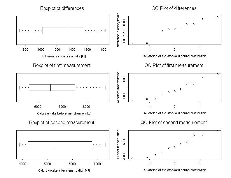
We return to the example of the calorie consumption. At first we take a look at the Q-Q-plot of the 11 measurements in figure 10.3.
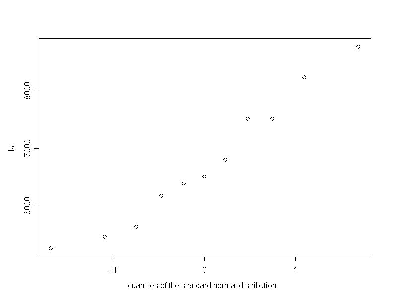
Since the points are scattered quite regularly along a straight line, we can hypothesize that the respective variable is close to normally distributed in the underlying population. Therefore we can test our alternative hypothesis that, on average, women consume less than \(7425\) kJ prior to their menstruation, using the \(t\)-test. This test allows us to decide whether or not to reject the null hypothesis \( H_0 : \mu \geq 7425 \,\text{kJ} \) in favour of the alternative hypothesis \( H_A : \mu \lt 7425 \,\text{kJ} \).
The test statistic \( t \) of the \(t\)-test is calculated from the difference between the sample mean \( 6753.6 \,\text{kJ} \) and \( \mu_0 = 7425 \,\text{kJ} \). This difference is \( -671.4 \,\text{kJ} \). It is divided by the standard error \( 344 = \frac{1140}{\sqrt{11}} \) (recall that the standard deviation of the 11 calorie values is \( 1140 \,\text{kJ} \). The test statistic \( t \) therefore takes the value \( -1.95 \).
What is the probability of such a low or an even lower value of the test statistic under the null hypothesis? In the preceding chapter we determined this probability, the so-called \(p\)-value with the applet "Type I error". However, the \(p\)-value however can also be found using Excel, via the function \(T.DIST(t;df;1)\). The number of degrees of freedom of \( t \) is \( n - 1 = 11 - 1 = 10 \). The resulting probability \( P(t_{df=10} \lt - 1.95) \) is found to be \(0.0399\). Thus the one-sided \(p\)-value of our result is \( 0.0399 \). Since this value is smaller than \(0.05\), we can reject the null hypothesis that, prior to their menstruation, women have an average daily calorie consumption of at least \(7425\) kJ, at the significance level \( \alpha = 0.05 \).
According to the central limit theorem (chapter 8), the condition that the variable in question be normally or at least close to normally distributed at the population level loses importance with increasing sample size. This leads to the following synopsis.
|
Synopsis 10.1.1
The one-sample \(t\)-test is suitable for comparing the mean of a variable \( X \) from a random sample to a reference value, provided that \( X \) is normally or close to normally distributed in the underlying population or if the sample size is sufficiently large. If the distribution of \(X\) is about symmetrical and there are no outliers, then a sample size \(\geq 15\) is generally sufficient (cf. [1], pp 397 ff). If the Q-Q-plot of \(X\) does not show very strong curvature, then \( n \geq 40 \) is generally sufficient (cf. [1}, pp 397 ff). The smaller the curvature of the Q-Q-plot, the smaller the sample size required for the one-sample \(t\)-test to be valid. If the distribution of \(X\) is very skewed and \(X\) only takes positive values, a logarithmic transformation of \(X\) may be warranted (cf. chapter 6). |
In a study concerning general anaesthesia conducted at the University Hospital Zurich [2], \(25\) patients were randomly chosen from a population of patients. These \(25\) patients were given the anaesthesia medication Propofol for their narcosis until the BIS (bispectral index) reached a certain value. Then the Propofol concentration was measured in the patients' blood plasma. The measured values are illustrated in the boxplot in figure 10.4.
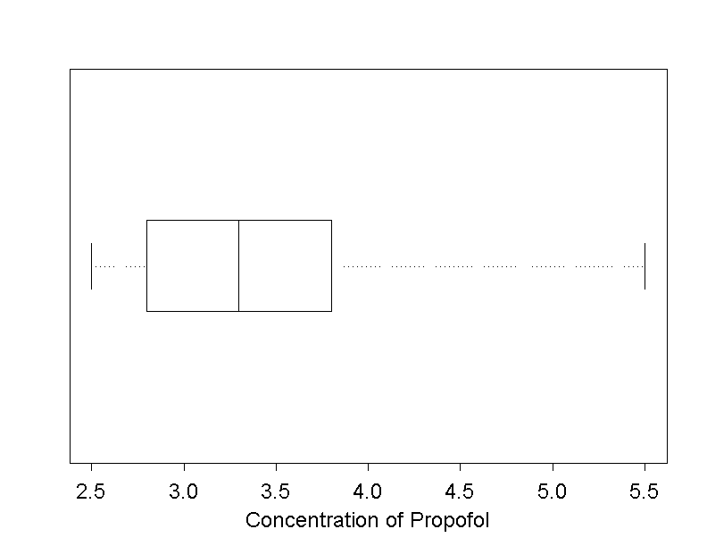
An empirical reference value for this concentration is \( 3.3 \,\text{mg/ml} \). We formulate the hypothesis that the mean of the attained propofol concentration in the patient population, from which the sample was drawn, differs from this reference value. In the language of statistics, we are interested in the following testing problem: \[ H_0 : \mu = 3.3 \,\text{mg/ml} \] against \[ H_A : \mu \neq 3.3 \,\text{mg/ml}.\]
The mean value of the \(25\) observations equals \( 3.42 \,\text{mg/ml} \). Is the deviation of this value from the reference value large enough to reject \( H_0 \)? We might use the one-sample t-test again to answer this question. However, we have to take a look at the Q-Q-plot of the measurements in figure 10.5.
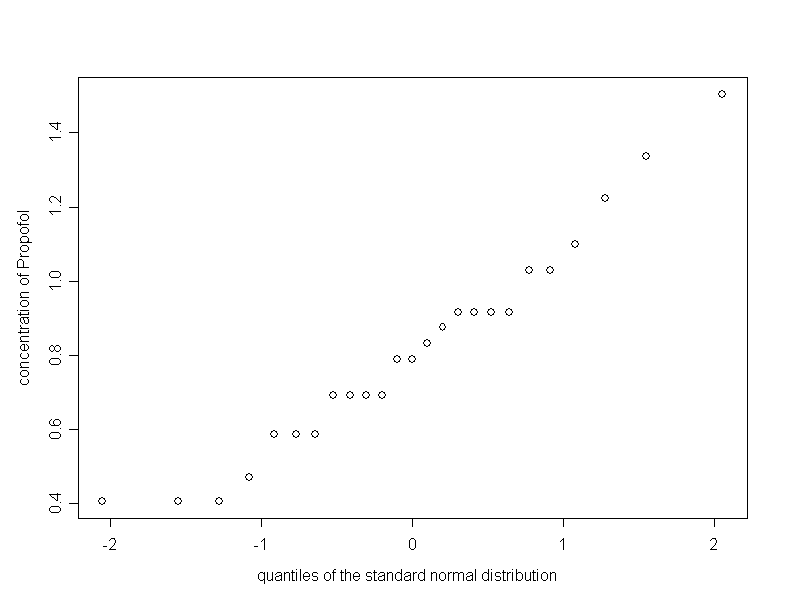
The Q-Q-plot raises some doubts that the data originate from a normal distribution. In particular, there are observations sharing the same value, which must be the result of rounding. The boxplot of the data indicates that the observations are approximately symmetrically distributed between the lower and the upper quartile, whereas the maximum and the minimum differ in their distance from the median. However this should not be overestimated when judging the symmetry, which is the condition for the Wilcoxon signed rank test. Generally, this test deals with differences. In our example, these are the differences of the individual measurements to the reference value \( 3.3 \,\text{mg/ml} \).
The null hypothesis of the signed rank test postulates that these differences are symmetrically distributed around \( 0 \) in the underlying population. To calculate the test statistic of the Wilcoxon signed rank test, the observed differences must be ranked. Therefore this test is also referred to as rank test. The ranking procedure is explained in the sequel.
|
Synopsis 10.2.1
The Wilcoxon signed rank test is suitable for the comparison of the mean of a variable \(X\) to a reference value, provided that \(X\) has a symmetrical yet not a normal distribution in the underlying population. |
For small sample sizes, the calculation of the \(p\)-value of the Wilcoxon signed rank test can be done using the exact distribution of the test statistic under \(H_0\). For larger sample sizes \(n\) it can be calculated using an approximation formula. These approximate \(p\)-values are quite accurate already for \( n \geq 15 \). The signed rank test can be performed in any statistics program, but not in Excel. The resulting two-sided \(p\)-value in our example is \(0.84\). At the end of the section, you can try to obtain an estimate of this \(p\)-value using the applet "Null distributions of sign and signed rank test".
To illustrate how the signed rank test works, we take the initial example of daily calorie consumptions of \(11\) women before their menstruation. However, in this case, we consider a two-sided alternative hypothesis \( H_A: \mu \neq 7425 \,\text{kJ}\). We this form the differences \( d_i = x_{i} - 7425 \) in the following table.
| \(x_{i}\) | \(d_i=x_{i} - 7425\) | \(|d_i|\) | rank of \(|d_i|\) | signed rank |
|---|---|---|---|---|
| 5260 | -2165 | 2165 | 11 | -11 |
| 5470 | -1955 | 1955 | 10 | -10 |
| 5640 | -1785 | 1785 | 9 | -9 |
| 6180 | -1245 | 1245 | 7 | -7 |
| 6390 | -1035 | 1035 | 6 | -6 |
| 6515 | -910 | 910 | 5 | -5 |
| 6805 | -620 | 620 | 3 | -3 |
| 7515 | 90 | 90 | 1.5 | 1.5 |
| 7515 | 90 | 90 | 1.5 | 1.5 |
| 8230 | 805 | 805 | 4 | 4 |
| 8770 | 1345 | 1345 | 8 | 8 |
Ranks are assigned to the absolute values of the differences in ascending order, i.e., the smallest difference gets rank \(1\) and the largest one rank \(n = 11\). If several observations share the same value, then their average rank is assigned to all of them. In our example, this applies to the two smallest differences which have the same value. As they would occupy ranks \(1\) and \(2\) if they were only minutely different, the mean of the two ranks, \(1.5\), is assigned to both. The signed ranks are obtained by putting a negative sign in front of ranks which were assigned to negative differences \(d_i \lt 0\). Differences equalling \(0\) are ignored in this test.
The sum of signed ranks, which is the test statistic of the signed rank test, equals \(-36\) in our example. Under the null hypothesis, we would, on average, expect a value close to \(0\). As the observed sum is quite different from \(0\), we may expect a small \(p\)-value. In fact, the two-sided \(p\)-value of this sum equals \(0.123\), as can be found using a statistics program. However, you may also use the applet "Null distributions of sign and signed rank test" to get a close estimate of this \(p\)-value. In this applet, you need to select "signed rank test" in the drop-down list, enter the number of differences \( \neq 0 \) and the observed sum of scores (which is the sum of signed ranks in case of the signed rank test).
In the Propofol-example, the sum of positive and of negative ranks equal \(170\) and \(-154\), respectively. Thus, the sum of signed ranks equals \(16\). As one of the differences equals \(0\), the number of differences \( \neq 0 \) equals \( n-1 = 25-1 = 24\). Try to determine the approximate \(p\)-value using the applet introduced in the next section.
Since the null hypothesis of the signed rank test involves the symmetry of the the distribution of the variable \( X \) in addition to the assumption about the mean value \(\mu\) of \(X\), the rejection of the null hypothesis may have two different implications, a) that we must reject the assumption that the distribution of \( X \) is symmetrical, or b) that we must reject the assumption that \( \mu \) equals the reference value in question.
The sign test provides an alternative, if we doubt the symmetry of the distribution of the variable \(X\). The null hypothesis of the sign test is that the median \( \tilde{\mu} \) of the distribution of \( X \) equals a reference value \( \tilde{\mu}_{0} \). The test statistic \( T \) of the sign test is obtained by determining the number \( n_{+} \) of positive difference \( (x_i - \tilde{\mu}_0) > 0\) and the number \( n_{-} \) of negative differences \( (x_i - \tilde{\mu}_0) \lt 0\).
Under the null hypothesis, the number \( n_{+} \) follows a binomial distribution with the parameters \( n = n_{+} + n_{-} \) and \( \pi = 0.5 \). If fact, if the null hypothesis is true, the numbers \( n_{+} \) and \( n_{-} \) must have the same expected values, which is the case if \( \pi = 0.5 \).
From figure 10.3. we can see that both \( n_{+} \) and \( n_{-}\) equal \(12\) in the example of . Thus, our result is in perfect agreement with the null hypothesis. If both numbers are the same, then the \(p\)-value must be 1, as the probability of observing a difference at least as large as 0 is 1. Differences equalling \(0\) are also ignored in the sign test.
|
Synopsis 10.3.1
If the sample size is small and the distribution of the differences between the observed values and the reference value in question appears to be skewed, then one can apply the sign test. Its null hypothesis states that the median of the differences equals \(0\). If this hypothesis is true, then the number of positive differences and the number of negative differences must be identical on average. Under the null hypothesis, the number of positive (resp. negative) differences follows a binomial distribution with the parameters \(n = \text{number of differences } \neq 0\) and \(\pi=0.5\). |
The sign and the signed rank test are illustrated by the Applet "Null distributions of sign and signed rank test".
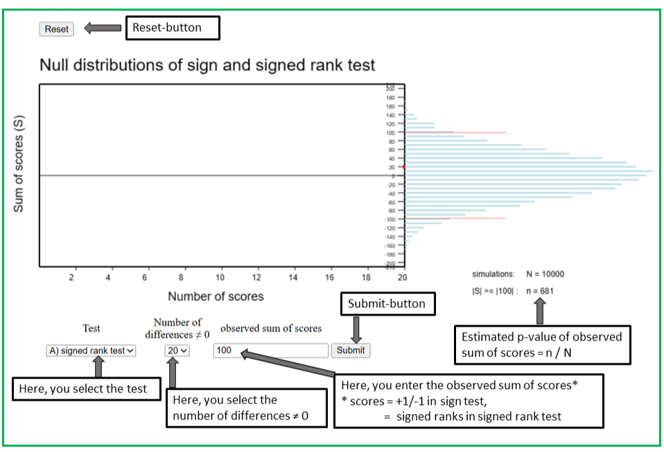
In the applet "Null distributions of sign and signed rank test", the distributions of the sum of scores of the sign and the signed rank test can be simulated under the respective null hypothesis. The scores of the sign test are the value 1 assigned to positive differences and the value -1 assigned to negative differences, while the scores of the signed rank test are the signed ranks of the positive and the negative differences.
A total of 10'000 sequences of n scores are simulated, where n denotes the number of differences unequal to 0 in the observed sample. The first five sequences are generated in slow motion and are displayed as moving blue trajectories showing how the sum of scores evolves across the n observations. The total sums of scores are represented as red dots, which disappear when the simulations continue at fast speed. The sequences 6 to 10'000 are not displayed, but their total sums appear as flashing red points.
On the right hand side of the panel, a frequency diagram grows. Each tiny blue dot represents 10 sequences with the respective total sum of scores. The simulations have ended if a new stable red dot appears.
To start the simulation, you must select the test in the first drop-down list and the number of differences unequal 0 in the second drop down list. The entry field "observed sum of scores" may be left empty. If you press "Submit", the simulation is started. If you have also entered the observed sum of scores S in the respective entry field, the number of simulated sums which are at least as distant from 0 as S will be displayed as soon as the simulations have ended. The ratio between this number and 10'000 is an estimate of the p-value of the observed score S. If you did not enter an observed value of S at the beginning, you can do this after the simulations have ended. Upon pressing "Submit", the results will be displayed. You can also replace the previously entered value of S by a new one and press "Submit" again to obtain an estimate of the p-value for this new value of S.
In a study concerning the eye disease "glaucoma" by H. Ehlers [3], the thickness of the cornea was measured in both eyes of \(8\) patients who had a healthy and a sick eye.
| Patient | Sick eye | Healthy eye | Difference |
|---|---|---|---|
| 1 | 488 | 484 | 4 |
| 2 | 478 | 478 | 0 |
| 3 | 480 | 492 | -12 |
| 4 | 426 | 444 | -18 |
| 5 | 440 | 436 | 4 |
| 6 | 410 | 398 | 12 |
| 7 | 458 | 464 | -6 |
| 8 | 460 | 476 | -16 |
We now have two measured values for each patient: \(x_{1,i}\) (sick eye) and \(x_{2,i}\) (healthy eye). The question of interest is whether or not the glaucoma disease has an influence on the thickness of the cornea. We therefore examine the differences \[ d_i = x_{1,i} - x_{2,i} \] in each patient. These differences are also listed in table 10.1. With these differences, we are back to a one-sample situation. We denote the population mean value of the cornea thickness of healthy eyes by \( \mu_H \) and the one of the sick eyes by \( \mu_S \). Moreover, we denote their difference by \( \mu_D = \mu_S - \mu_H \). Our question is translated into the null hypothesis \( H_0 : \mu_D = 0 \) (respectively \( H_0 : \mu_S = \mu_H \)) and the alternative hypothesis \( H_A : \mu_D \neq 0 \) (respectively \( H_A : \mu_S \neq \mu_H\)).
To decide whether to use the \(t\)-test or not, we take a look at the Q-Q-plot of the differences in cornea thickness in figure 10.6.
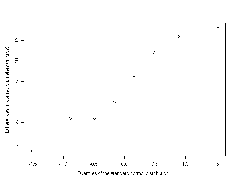
We get the impression that the distribution of these differences does not deviate much from a normal distribution. Therefore, we apply a two-sided \(t\)-test. The mean value of the observed differences equals \( -4 \) and the standard deviation \( 10.744 \). Therefore the standard error of the mean equals \( \frac{-4}{\sqrt{8}} = -1.053 \). If we had a one-sided test as before, the \(p\)-value would be \( P(t_{df=7} \lt -1.053) = 0.164 \). This value is obtained in Excel using \(T.DIST(-1.053;7;1)\). If the \(t\)-value had been positive, then we would have had to take \(1 - T.DIST(t;7;1)\). However, as we have a two-sided alternative hypothesis, this value must be doubled (to take into account equal deviations from \(0\) in both directions. Thus, we obtain a \(p\)-value of \(0.33\) and can not reject the null hypothesis. The hypothesis that the glaucoma disease has an influence on the thickness of the cornea is thus not sufficiently supported by our data. However, we have to consider that the test had little power given the small sample size of \( n = 8 \). Furthermore the assessment of the normal distribution assumption is quite problematic with only \(8\) observations. In case of doubt it is advisable to use the Wilcoxon signed rank test or the sign test instead.
The term "paired t-test" is generally used if pairwise measurements are to be compared using the t-test. When running the paired t-test in a statistics program, one must indicate the two paired variables to be compared. In the background, the program then calculates the differences of the two variables within pairs and applies the one-sample t-test to the differences, as we did in the previous example.
|
Synopsis 10.4.1
In the case of two paired samples we can get back to the one-sample case by computing the differences within pairs. |
In chapter 8, you have learned how to calculate a \(95\%\)-confidence interval for a population mean using the \(t\)-distribution. For the glaucoma data we get \( [-12.98\mu m, 4.98\mu m]\) as \(95\%\)-confidence interval of the population mean value \( \mu_D \) of the paired differences. Instead of performing the two-sided \(t\)-test at the level \( \alpha = 5\% \), we can check whether or not \( 0 \) is contained in the \(95\%\)-confidence interval. In our case \(0\) lies in the confidence interval. Therefore we cannot reject \(H_0\) at the significance level \( \alpha = 5\%\). If \(0\) did not lie in the confidence interval, the result would be statistically significant at the \(5\%\)-level and would argue in favour of the alternative hypothesis.
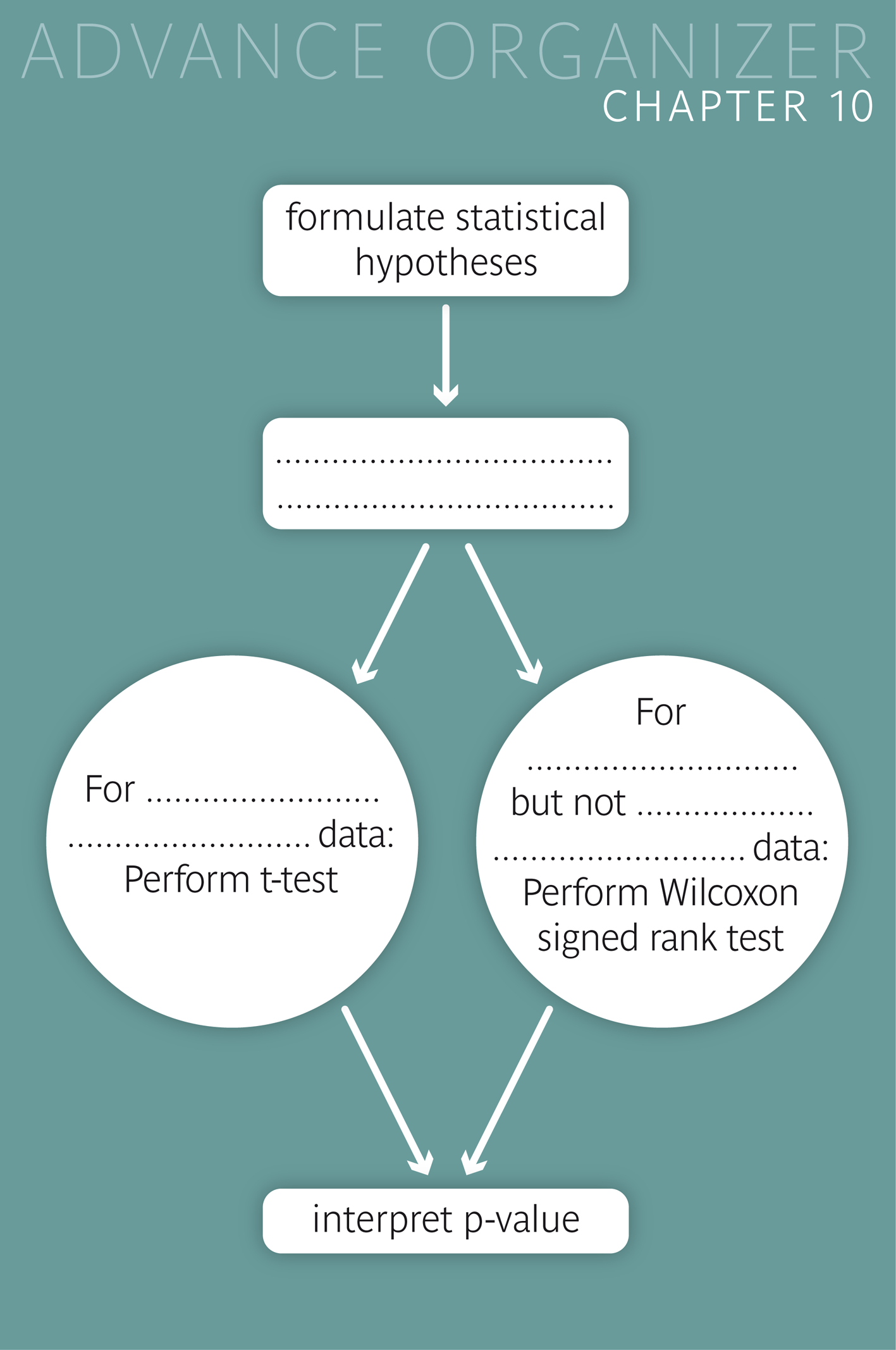
A sample mean can be compared to a hypothetical mean \( \mu_0 \) by means of the one-sample \(t\)-test or the Wilcoxon signed rank test. Based on the question of interest we first have to formulate the hypotheses. We distinguish between three testing situations: one situation with a two-sided alternative hypothesis and two situations with a one-sided alternative hypothesis.
We use the Q-Q-plot to evaluate whether the distribution of the relevant differences is approximately normal. If this is the case, or if the sample size is large, we can apply the \(t\)-test. However, if the Q-Q-plot argues against a normal distribution or if we do not have enough data to reliably interpret it, we may apply the Wilcoxon signed rank test with small to medium sample sizes, provided that the distribution of the differences is approximately symmetrical. The conditions for the Wilcoxon signed rank test are therefore less restrictive for small to medium sample sizes than the ones for the \(t\)-test.
We summarise the information of the data in a test statistic that measures the "distance" of the sample result to the null hypothesis. Under the assumption that the null hypothesis applies, we then calculate the probability of observing at least the same difference again in another random sample of the same size from the same population. Based on this probability, the so-called \(p\)-value, we can decide whether or not to reject the null hypothesis at the pre-specified significance level \(\alpha\).
The same tests can also be applied when comparing the means of two paired samples because we get back to the one-sample situation when computing the differences of the measurement values within pairs.
In order to assess the statistical significance of a difference at the 5%-level, we can also consider the 95%-confidence interval of the respective test statistic. The mean values of two paired samples differ significantly at the level of 5% if and only if the 95%-confidence interval of the mean of the paired differences does not include \(0\).
If the sample size is small and the differences seem to have a skewed distribution, then one can apply the sign test. Its null hypothesis states that the median of differences is \(0\) at the population level. Unlike the t-test and the Wilcoxon signed rank test, this test has no validity conditions.
[1] D.S. Moore, G.P. McCabe, B.A. Craig
Introduction to the practice of Statistics
10th edition, 2021
Macmillan International, Higher Education, New York
[2] S.B. Fehr, M.P. Zalunardo, B. Seifert, K.M. Rentsch, R.G. Rohling, T. Pasch, D.R. Spahn (2001)
Clonidine decreases propofol requirements during anaesthesia: effect on bispectral index.
British Journal of Anaesthesia, 86 (5), 627-32.
[3] N. Ehlers (1970)
On corneal thickness and introcular pressure II
Acta Opthalmologica, 48, 1107-12
Data copied from p. 127 of
D.J. Hand, F. Daly, A.D. Lunn, K.J. McConway, E. Ostrowski
Handbook of Small Data Sets
Chapman and Hall, London, 1994