|
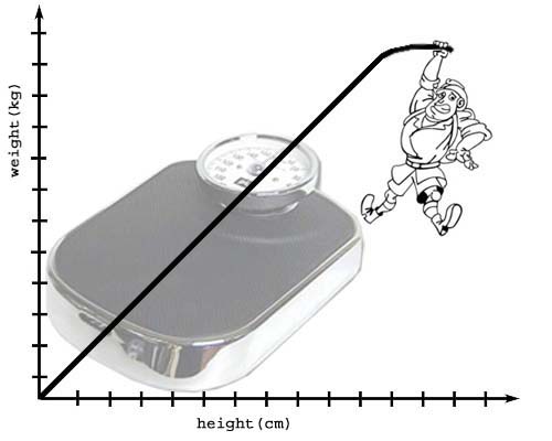
How can a doctor estimate the blood volume of a patient without extensive measurements, or how can he judge if the lung function values of a patient are within the norm for his/her age? Regression models are an elegant tool to answer such questions. |
|
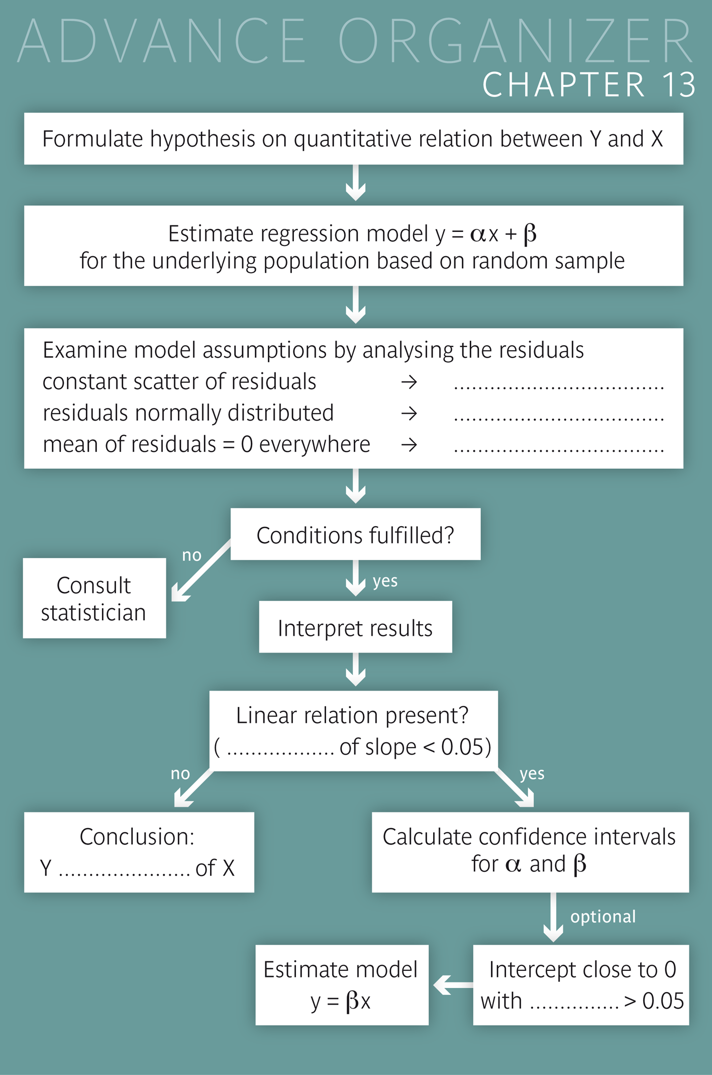
Educational objectives You can explain in your own words what a regression line tells about the relation between a dependent variable \(Y\) and an independent variable \(X\) and what the residuals mean. You are familiar with important properties of the regression line and you can explain how regression lines are defined. lines from other lines. You can correctly interpret the parameters of the regression line (slope and intercept) in concrete examples. You are able to judge if a straight-line model is suitable for the description of a quantitative relation. You are familiar with the conditions which must be fulfilled in order for the standard errors of the regression parameters to be estimated correctly. You can extract and interpret the most important information from a regression output provided by a statistics program. In particular you will be able to judge the statistical significance of a parameter estimate and interpret it correctly. You will also be able to calculate confidence intervals for the regression parameters based on the information in the regression output. Key words: regression line, regression parameter, intercept, slope, residuals, regression equation, regression model, model assumptions, residual plo Previous knowledge: scatter plot (chap. 2), sample mean (chap. 3), population parameters (chap. 4), normal distribution, Q-Q plot (chap. 6), standard error, confidence interval (chap. 8), statistical hypothesis, statistical test, \(p\)-value (chap. 9) Central questions: When does it make sense to describe the relation between a variable \(Y\) and a variable \(X\) by a regression line model? How does such a model have to be interpreted and under which conditions is it valid? |
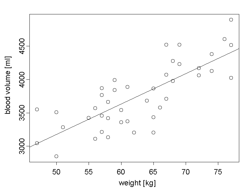
The following table shows the body weight and blood volume of \(42\) adult women. Underneath the table, the relation between these two variables is illustrated in a scatter plot. Each point of the diagram represents one person. The weight of the person defines the x-coordinate of the point and the blood volume the y-coordinate.
| Weight [kg] | Blood volume [ml] | Weight [kg] | Blood volume [ml] | |
|---|---|---|---|---|
| 47 | 3552 | 57 | 3764 | |
| 56 | 3567 | 74 | 4128 | |
| 57 | 3211 | 76 | 4605 | |
| 77 | 4897 | 64 | 3683 | |
| 65 | 3863 | 50 | 2845 | |
| 77 | 4026 | 65 | 3431 | |
| 47 | 3042 | 55 | 3424 | |
| 72 | 4062 | 58 | 3419 | |
| 68 | 3974 | 67 | 4520 | |
| 57 | 3869 | 69 | 4520 | |
| 51 | 3281 | 65 | 3205 | |
| 69 | 4232 | 50 | 3508 | |
| 66 | 3579 | 68 | 4275 | |
| 77 | 4516 | 60 | 3358 | |
| 58 | 3662 | 67 | 3709 | |
| 72 | 4170 | 56 | 3112 | |
| 58 | 3133 | 74 | 4382 | |
| 67 | 4069 | 61 | 3371 | |
| 62 | 3204 | 59 | 3993 | |
| 57 | 3455 | 60 | 3541 | |
| 61 | 3889 | 59 | 3840 |
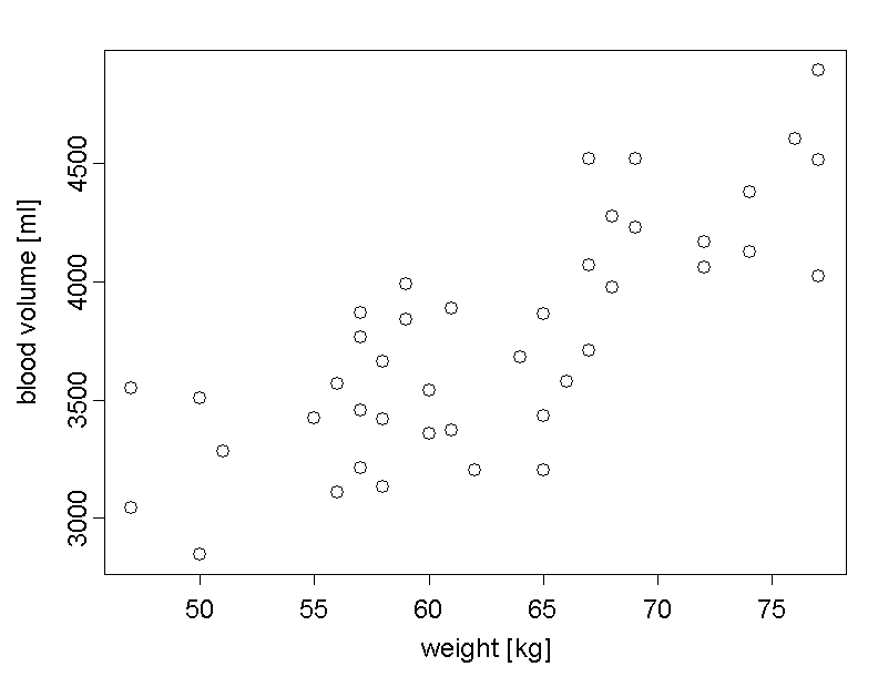
We notice that the point cloud increases if we move from left to right. Hence, heavier people tend to have higher blood volumes than lighter people.
In the applet "Scatter plot and regression line" you can find the scatter plot of the blood volume and body weight of the \(42\) women.
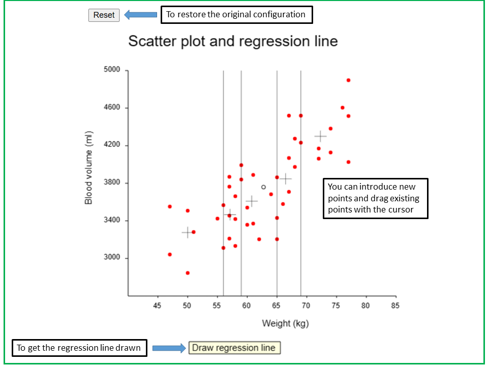
In the applet "Scatter plot and regression line", the scatter plot of blood volume vs. weight of the 42 women is drawn.
The plot is divided into 5 sectors with about the same number of points. In each of the sectors, the centre of gravity (i.e., defined by the mean values of weight and blood volume) is drawn as a grey reticle. You can see that these reticles are lined up pretty much along a straight line.
By pressing the key "Draw regression line", the regression line will be drawn into the scatter plot. Indeed, the 5 reticles are close to this straight line.
You can also add points by clicking the cursor and drag points with the cursor. The reticles and the regression line will change accordingly. By pressing the reset-button in the upper left corner, the original configuration can be restored.
The data are divided into \(5\) classes with about equal numbers of points along the \(x\)-axis, and each of the \(5\) reticles indicates the centre of gravity of the points contained in the respective class.
We can see that the reticles lie roughly on a straight line. Therefore we can assume a linear relation between the mean blood volume of adult women and their body weight. We are thus looking for a straight line which best possibly describes this relation. Depending on the definition of "best possible", we get different mathematical solutions. However, we will only treat the classical definition, which has the best mathematical properties in many situations and which provides the classical regression line.
If we simply speak of "the regression line" in the sequel, we always mean this classical solution. The mathematical definition of the regression line will be provided later. When pressing the button "Draw regression line" of the applet, the regression line will be drawn into the scatter plot. You will notice that it indeed almost hits the \(5\) reticles.
The scatter plot of blood volume vs. weight with the sssociated regression line is also provided in the following figure:
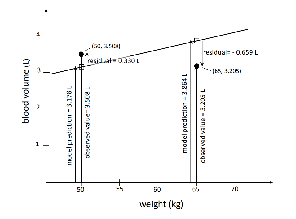
Each individual point deviates more or less strongly from the regression line. The deviations of the individual points from the line are called "residuals". It is important to emphasize that these deviations are not measured perpendicularly to the line, but in the direction of the y-axis. Two of the \(42\) points and their residuals are illustrated in the following diagram.
In the so-called "residual plot", the residuals are plotted against the values of the independent variable (body weight in our case):
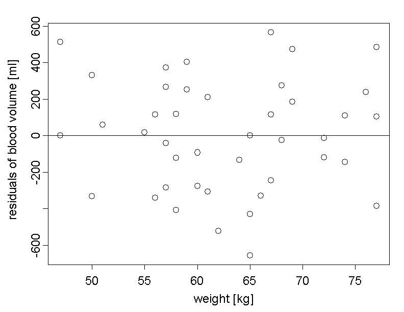
On average, the positive and negative residuals cancel out so that their mean value is \(0\).
The scatter plot of the data and the residual plot are also illustrated in the applet "Regression line and residual plot". You can add new data points and move existing points with the cursor and observe how the regression line and the residual plot change. With the reset-button, you can restore the original configuration.

In the applet "Regression line and residual plot", the scatter plot of blood volume vs. weight of the 42 women and the regression line are drawn in the upper part of the panel,
In the lower part of the panel, the residual plot is represented. As in the preceding applet, the x-axis is divided into 5 sectors with about equal numbers of points. Now, in each sector, there is a reticle for the original points and a reticle for the residuals. Both are defined by the center of gravity of the respective points. The y-coordinate of the upper reticle is the mean value of blood volume, while the y-coordinate of the lower reticle is the mean value of residuals. These reticles are close to the x-axis, as the mean values of residuals should be close to 0 in different segments if the dependency of the mean value of Y on X is close to linear.
You can also add points by clicking the cursor and drag points with the cursor. The residuals, the regression line and the reticles will change accordingly. By pressing the reset-button in the upper left corner, the original configuration can be restored.
Note: This applet will be used again in the following section.
In our example, "weight" has the role of the independent or explanatory variable and blood volume has the role of the dependent variable. The regression line describes the relation between the mean of blood volume and body weight of women in a model. We therefore generally speak of regression models. A "regression model" provides a prediction of the value of the dependent variable \(Y\) for each value \(x\) of the explanatory (or independent) variable \(X\).
|
Definition 13.1.1
In general, the independent variable is denoted by \(X\) and the dependent variable by \(Y\) in a regression model. The terms "explanatory variable" or "predictor variable" are also commonly used for \(X\), and \(Y\) is often also called "response variable" or "outcome variable". The difference between the observed value of \(Y\) (denoted \(y_{obs}\)) and the value predicted by the regression model (denoted \(y_{pred}\)) is called "residual" of the respective observation. If the regression model is applied to observations, which do not belong to the sample from which it was derived, then we speak of prediction errors instead of residuals. The prediction error is defined as \(y_{pred} - y_{obs}\), unlike the residual which is defined as \(y_{obs} - y_{pred}\). |
|
Synopsis 13.1.1
If the mean of a variable \(Y\) depends approximately linearly on the value of another variable \(X\), then this dependency can be described by the model of a regression line. In the sample from which the regression line was derived, the mean value of the residuals equals \(0\). This should also approximately hold for the prediction errors arising if a regression model is used to predict \(Y\) in future observations. Independent of the value of the explanatory variable \(X\), the prediction errors should cancel out (i.e., have a mean value close to \(0\) in a longer series of predictions. |
We should always ask this question early on when trying to estimate a regression model.
If the relation is not linear in reality, a straight-line model does not make much sense. In order to judge if the mean of the blood volume indeed increases linearly with the body weight, we can again take a look at the residual plot. If the relation were not linear, the scatter plot of the residuals would not be horizontal but rather curved or undulated.
We can often see this better if we examine the mean values of the residuals in several sections of the independent variable. If they vary randomly around the \(0\)-line, we can assume that the relation is essentially linear. But if these points follow a "banana shape" or a simple wave shape (with a crest and a trough), then the linearity of the relation must be questioned.
In the applet "Regression line and residual plot", the scatter plot of blood volume vs. weight of the 42 women and the regression line are drawn in the upper part of the panel,
In the lower part of the panel, the residual plot is represented. As in the preceding applet, the x-axis is divided into 5 sectors with about equal numbers of points. Now, in each sector, there is a reticle for the original points and a reticle for the residuals. Both are defined by the center of gravity of the respective points. The y-coordinate of the upper reticle is the mean value of blood volume, while the y-coordinate of the lower reticle is the mean value of residuals. These reticles are close to the x-axis, as the mean values of residuals should be close to 0 in different segments if the dependency of the mean value of Y on X is close to linear.
You can also add points by clicking the cursor and drag points with the cursor. The residuals, the regression line and the reticles will change accordingly. By pressing the reset-button in the upper left corner, the original configuration can be restored.
Try to obtain different shapes of the residual plot ("banana", "wave") by adding data points to the scatter plot.
Now restore the original plot by clicking on the reset-button.
Try to answer the following question.
There are also formal methods for judging whether or not the linearity assumption is justified. However, they are relatively complex and cannot be treated within the scope of this course.
We conclude this section with an example in which the relation between \(Y\) and \(X\) is not described correctly by a straight line [1].
The dependency of the diameter and the surface area of the cornea on age was examined in fetuses.

We can see from the curvature of the scatter plot in diagram A of figure 13.9 that the mean diameter of the cornea does not linearly depend on age. The solid line shows an estimate of the true relation based on a quadratic function of age. The respective curve is defined by the equation [1] \[\text{mean diameter} = -1.6 + 4.256 \times \text{age} - 0.039 \times \text{age}^2 .\] The term with the square of age captures the curvature of the relation.
In diagram B of figure 13.9 we can see that the relation between the mean surface area of the cornea and age can be well described by a straight line, since no curvature can be observed. The corresponding regression line is given by the equation [1] \[\text{mean surface area} = -22.620 + 2.302 \times age .\]
Exercise:
Think about examples from Medicine in which non-linear relations occur or might occur.
From high school you will remember that a straight line is given by the equation \[y = \alpha + \beta \times x , \] Here, the parameter \(\beta\) denotes the slope of the straight line (slope parameter) and the parameter \(\alpha\) denotes the point at which the straight line intersects the y-axis, i.e., the vertical line at \(x = 0\) (intercept parameter).
If the relation between the mean value of \(Y\) and \(X\) is linear in the population from which the random sample was drawn, then this relation can be described by the above equation. In our example, \(Y\) stands for the blood volume and \(X\) for body weight. We do not know the values of \(\alpha\) and \(\beta\), but we can estimate them based on the regression line from our random sample.
The intercept of the observed regression line is generally denoted by \(\hat{\alpha}\) and its slope by \(\hat{\beta}\). These values are estimates of \(\alpha\) and \(\beta\).
Notice that estimates of a population parameter \(\Theta\) are generally denoted by \(\hat{\Theta}\), i.e., by equipping the parameter with a hat.
|
Synopsis 13.3.1
The regression line \(y = \alpha + \beta \times x\) at the population level is determined by the two parameters \(\alpha\) and \(\beta\), which are estimated from the data of a random sample. The parameter \(\beta\) indicates the slope of the regression line (\( = \Delta y / \Delta x)\)) and the parameter \(\alpha\) indicates at which point the regression line intersects the y-axis. The estimates of \(\alpha\) and \(\beta\) from the sample are denoted by \(\hat{\alpha}\) and \(\hat{\beta}\). They are generally referred to as "parameter estimates". |
In our example we get the following estimates for the slope and the intercept of the regression line: \[\hat{\beta} = 45.7 \, ,\] \[ \hat{\alpha} = 893 \, . \]
We now want to look at the mathematical properties of the regression line. They are summarised in the following synopsis.
|
Synopsis 13.3.2
The regression line has the following important properties:
|
The so-called "least squares method" which is used to determine regression lines was already introduced about 200 years ago by the famous German mathematician Karl Friedrich Gauss.
In the following applet, you can observe how a straight line can be fitted to the data using the least squares method.

With the applet "Minimize the residual variance" you can try to find the regression line yourself. You can move the line up or down with the cursor positioned near the center, and you can change the slope of the line by moving its ends up or down with the cursor. Initially, the bar underneath the scatter plot is colored in black. If you move the line slowly upwards, the color of the bar will suddenly turn red. This happens when the y-coordinate of the line gets very close to the mean of blood volume. Now, the variance of the residuals equals the variance of blood volume. This means that the regression line does not explain any of the variability of blood volume. Accordingly, the value of "R-squared current line" is 0. The horizontal line at the level of the mean value of Y is referred to as null-model.
If the bar is red and you start to rotate the line in the direction of the scatter plot, then a green bar appears on the left hand side and pushes the red bar back. You have found the regression line, if the green bar reaches the black vertical line within the red part of the bar. This is as far as you can get. In this case, the R-squared of your line equals 0.604 (the proportion of variance of blood volume explained by the regression line).
The green (red) part of the bar represents the proportion of the variance of blood volume which is (is not) explained by the current line.
Whenever the variance of the residuals gets larger than the variance of the blood volume, the bar turns black. Such a model would be worse than the null-model. As in the null-model, the proportion of the variance of blood volume explained by such a line is 0.
By pressing the reset-button in the upper left corner, the original configuration can be restored.
You can find the regression line of our example yourself with the applet "Minimise the residual variance", by rotating and shifting the straight line until it has reached its optimal position.
This position is characterised by the property that the variance of the residuals (red bar) is minimised. In the original position, the straight line runs horizontally in the lower part of the scatter plot. If you move the line slowly upward with the cursor (i.e., by seizing it near the center), the horizontal bar underneath will turn red as soon as the \(y\)-coordinate of the line gets close to \(\bar{y}\).
A horizontal line at the level \(\bar{y}\) represents the so-called "null model". In the null-model, the residuals are exactly equal to the differences between the individual observations \(y_i\) and \(\bar{y}\). Therefore they have the same variance as the observations \(y_i\) themselves. Hence, the null-model does not explain any of the variance of the \(y_i\).
If the bar is black, the variance of the residuals is even larger than the variance of the \(y_i\). These models are thus worse than the null model.
If the line is close to the null model and you rotate it in the direction of the scatter plot (by seizing it at the right or left end), then a green bar appears to the left and the red bar gets shorter. The green bar corresponds to the proportion of the variance of the \(y_i\)-values, which is explained by the line. The optimal position is reached if the green bar reaches the vertical black line within the red bar.
Additional information for maths or physics enthusiasts:
If the residuals were forces which act on the regression line (positive residuals = vertical upward forces, negative residuals = vertical downward forces), then the line would be in an equilibrium state, since the sum of the forces and the sum of the torsional moments would both be \(0\).
Below you can see an example of a regression output by a statistics program for our example:
Analysis of Variance
| Source | DF | Sum of Squares | Mean Square | F Value | Pr > F |
|---|---|---|---|---|---|
| Model | 1 | 5810017 | 5810017 | 61.07 | \(\lt 0.0001\) |
| Error | 40 | 3805658 | 95141 | ||
| Corrected Total | 41 | 9615675 |
| Root MSE: | 308.45008 | R-Square: | 0.6042 |
|---|---|---|---|
| Dependent Mean: | 3759.25277 | Adj R-Sq: | 0.5943 |
| Coeff Var: | 8.20509 |
Parameter Estimates
| Variable | DF | Estimate | Standard Error | t-Value | Pr \( \gt |t|\) |
|---|---|---|---|---|---|
| Intercept | 1 | 893.25323 | 369.82725 | 2.42 | 0.0204 |
| Weight | 1 | 45.68197 | 5.84576 | 7.81 | \( \lt 0.0001\) |
In the following, we will mainly the address the lower part of the output.
We will first focus on the lower part with the title "Parameter Estimates". In the first column, we can see the already familiar estimates of the intercept (level at which the line intersects the \(y\)-axis) and the slope (here denoted by "Weight").
In the second column, estimates of the standard errors of the two parameter estimates are listed. Like all sample estimates, \(\hat{\alpha}\) and \(\hat{\beta}\) also vary from one random sample to another. The standard error of \(\hat{\beta}\) (i.e. the standard deviation of the estimates of \(\beta\) in repeated samples of equal size from the same population) is estimated at \(5.8\) ml/kg in our example. This estimate can be calculated relatively easily with the formula of the following synopsis.
|
Synopsis 13.4.1
The estimate of the standard error of \(\hat{\beta}\) (slope of the observed regression line) is calculated as follows: \[ SE(\hat{\beta}) = \frac{\text{standard deviation of residuals}}{\sqrt{n - 1} \times \text{(standard deviation of x-values)}}\] |
Strictly speaking, we should also put a hat on \(SE\), as this is an estimate of the true standard error of \(\hat{\beta}\). To calculate the true value of \(SE(\hat{\beta})\), we would need to know the standard deviation of the residuals at the population level.
Exercise:
Try to calculate the standard error of \(\hat{\beta}\) yourself with the formula above. Note: The standard deviation of the \(x\)-values is \(8.2\) kg in our example and the standard deviation of the residuals is \(308\) ml. The latter value appears in the regression output above. It is the so-called "Root MSE" (i.e., the root of the "mean squared error" or - which is the same - the root of the variance of the residuals).
Here we can again recognise the "square root of \(n\) law" (with the slight difference that the denominator contains the square root of \(n - 1\) instead of the square root of \(n\)).
It is not surprising that the standard error of \(\hat{\beta}\) directly depends on the standard deviation of the residuals.
On the other hand, it is inversely proportional to the standard deviation of the \(x\)-values. This is due to the fact that points which are far away from the centre in the direction of the \(x\)-axis, have a stabilising effect on the slope of the regression line. This can be compared to a board which is propped on two blocks. The stability of the board increases with the distance of the two blocks.
The \(95\%\)-confidence interval for the slope \(\beta\) of the regression line in the population is calculated as follows: \[\hat{\beta} \pm t_{0.975,n-2} \times SE(\hat{\beta}),\] where \(n\) denotes the sample size and \(t_{0.975,n-2}\) is the \(97.5\)-th percentile of the \(t\)-distribution with \(n-2\) degrees of freedom. Notice that each estimated parameter reduces the number of degrees of freedom by \(1\). The number of degrees of freedom of the observed data is \(n\). However, as we estimated the parameters \(\alpha\) and \(\beta\), the number of degrees of freedom in the residuals equals \(n-2\).
With large sample sizes, the \(97.5\)th percentile of the \(t\)-distribution can be replaced by the factor \(1.96\) (the \(97.5\)th percentile of the standard normal distribution).
In order for the confidence interval to be valid (i.e. to cover the value \(\beta\) of the regression line at the population level in \(95\%\) of all cases), the following four conditions have to be fulfilled:
Conditions 1 to 3 must be fulfilled even in large samples. If this is not the case, the confidence interval calculated according to the above formula is biased.
On the other hand, condition 4 loses importance with increasing sample size and can be ignored if the sample size is large.
In order to check conditions 1 and 2, we can use the applet "Regression line and residuals with boxplots".

The applet "Regression line, residuals and boxplots" resembles the applet "Regression line and residual plot". However, in this applet, the reticles are replaced by boxplots in the direction of the y-axis. Thus, the boxplots in the upper part of the panel describe the distribution of blood volume in the respective segments, while those in the lower part of the panel describe the distribution of residuals in the respective segments.
For a regression model to be valid, the variability of residuals should be about constant across the entire x-axis. The boxplots of residuals should therefore have about the same interquartile range in all segments. In particular, the variability of residuals must not show a systematic increase or decrease if one moves from left to right on the x-axis.
You can again add points by clicking the cursor and drag points with the cursor. The residuals, the regression line and the boxplots will change accordingly. By pressing the reset-button in the upper left corner, the original configuration can be restored.
In the applet "Regression line, residuals and boxplots", the boxplots of the original blood volumes and of the residuals are drawn for five different intervals across the \(x\)-axis.
Answer the following question with the applet.
If there are correlations between individual observations, then the third condition is usually violated. This is the case if all or some observational units contribute more than one observation or if the observations can be grouped based on familal, social or geographic relations. This also generally holds true for time series data, where the observational units are consecutive time periods (e.g., for the daily number of emergency admissions in a county hospital or for the annual number of new lung cancer cases in a specific country).
The regression equation along with the model assumptions constitute the so-called "regression model". The classical regression model thus requires that the residuals be normally distributed, have a mean value of \(0\) and a constant scatter within the range of \(X\), and be independent of one another.
|
Synopsis 13.5.1
The \(95\%\)-confidence interval for the slope \(\beta\) of the regression line at the population level is calculated as follows: \[\hat{\beta} \pm t_{0.975,n-2} \times SE(\hat{\beta}) , \] where \(\hat{\beta}\) denotes the estimate of \(\beta\) and \(SE(\hat{\beta})\) the estimate of the standard error of \(\hat{\beta}\), \(n\) the sample size and \(t_{0.975,n-2}\) the \(97.5\)th percentile of the \(t\)-distribution with \(n - 2\) degrees of freedom. In order for this confidence interval to include the value \(\beta\) in \(95\%\) of all cases, the following conditions have to be fulfilled:
|
If we can assume that the mean value of \(Y\) is either not dependent of \(X\) at all or depends linearly on \(X\), then we should be able to answer this question.
We will now examine the third and fourth column of the regression output in more detail. In the third column, the \(t\)-values of the parameter estimates are listed. The \(t\)-value of a sample statistic is defined as the ratio between the sample statistic and its standard error estimate. The \(t\)-value of \(\hat{\beta}\) is thus given by \[t = \frac{\hat{\beta}}{SE(\hat{\beta})} .\] The absolute value of \(t\) indicates the number of standard errors separating \(\hat{\beta}\) from \(0\).
The larger the value of \(|t|\) , the less plausible the null hypothesis \(\beta = 0\). The following synopsis shows which values of \(t\) lead to a rejection of the null hypothesis at the common significance level of \(5\%\).
|
Synopsis 13.7.1
If the mean value of \(Y\) depends linearly on \(X\) or is unrelated to \(X\), then the hypothesis that the slope \(\beta\) of the regression line differs from \(0\) can be tested as follows: If the absolute value of \(t = \frac{\hat{\beta}}{SE(\hat{\beta})}\) is larger than \(t_{0.975,n-2}\), then the null hypothesis \(\beta = 0\) is rejected at the significance level of \(5\%\). In this case, \(\hat{\beta}\) is said to be significantly different from \(0\) or just to be statistically significant at the \(5\%\)-level. If the null hypothesis cannot be rejected, then the observed data do not (or not sufficiently) support the hypothesis of a linear relation between the mean of \(Y\) and \(X\). |
Of course we are mostly interested in the \(p\)-value of \(\hat{\beta}\) (by this we mean the \(p\)-value of the difference between \(\hat{\beta}\) and \(0\)). It is calculated on the basis of the \(t\)-value. In chapter 10, we have already seen how this can be achieved using EXCEL. Denoting the observed \(t\)-value by \(t_{obs}\), the \(p\)-value is obtained using the formula \[p = 2\times(1-T.DIST(|t_{obs}|;n-2;1)) ,\] where the EXCEL-function \(T.DIST(c;df;1)\) gives the probability of a \(t\)-value \(\lt c\) under the \(t\)-distribution with \(df\) degrees of freedom. In our example, the number of degrees of freedom equals \(n-2 = 40\).
The point \((0,0)\) if commonly called the origin of the coordinate system.
If the null hypothesis \(\alpha = 0\) were not rejected, we could estimate a new regression line running through the origin of the coordinate system. Such regression lines however do not have the nice property that they pass through the centre of gravity \((\bar{x}, \bar{y})\) of the data.
|
Synopsis 13.8.1
If the mean value of \(Y\) linearly depends on \(X\), then the hypothesis that the regression line does not pass through the origin \((0, 0)\) can be tested as follows: If the absolute value of \(t = \hat{\alpha}/SE(\hat{\alpha})\) is larger than \(t_{0.975,n-2}\), then the null hypothesis \(\alpha = 0\) must be rejected at the level of \(5\%\). In this case, \(\hat{\alpha}\) is said to be significantly different from \(0\) or statistically significant at the level of \(5\%\). If the null hypothesis can not be rejected, the data do not (or not sufficiently) support the hypothesis that the regression line at the population level does not pass through the origin. |
Since the two parameter estimates \(\hat{\alpha}\) and \(\hat{\beta}\) differ randomly from the true parameters \(\alpha\) and \(\beta\) at the population level, \(\hat{\alpha} + \hat{\beta} \times x\) differs randomly from the respective \(y\)-value \(\alpha + \beta \times x\) of the true regression line at any point \(x\). Therefore the \(95\%\)-confidence interval for \(\alpha + \beta \times x\) should be plotted at each value of \(x\).
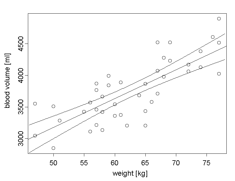
We notice that the confidence interval is narrowest in the centre and becomes wider with increasing distance from the centre. This is due to the fact that the sampling error of the slope has an ever stronger influence with increasing distance from the centre. In the centre, the confidence interval is only determined by the uncertainty regarding \(\bar{y}\).
A common misinterpration:
It is not true that the area between the two curves fully covers the regression line at the population level in \(95\%\) of all cases. This coverage property only holds for individual points of the regression line, but not for multiple points.
|
Synopsis 13.9.1
For each value \(x\), the respective \(y\)-value of the empirical regression line defines an estimate of the respective \(y\)-value of the true regression line at the population level. The \(95\%\)-confidence interval of this estimate is getting wider with increasing distance between \(x\) and \(\bar{x}\). Hence it is narrowest where \(x = \bar{x}\). This is due to the fact that points on the regression line farther away from the centre are moved up or down more strongly with the sampling error of the regression slope than points which are located close to the centre. |
If the mean value of a variable \(Y\) linearly depends on another variable \(X\), then this relation can be described by a regression line. For each value \(x\) of \(X\), this line provides an estimate of the mean (or expected) value of \(Y\) given \(X = x\).
The regression line is determined by the sample data of \(Y\) and \(X\), and it has the property of minimising the variance of the residuals (i.e., the differences between the observed and the predicted \(y\)-values). The regression line is given by the formula \[y = \hat{\alpha} + \hat{\beta} \times x , \] where the coefficients \(\hat{\alpha}\) (intercept of the regression line with the \(y\)-axis) and \(\hat{\beta}\) (slope of the regression line) are estimates of the respective parameters \(\alpha\) and \(\beta\) of the regression line at the population level.
\(95\%\)-confidence intervals for \(\alpha\) and \(\beta\) are calculated from their sample estimates and the respective standard error estimates, by multiplying the standard error estimates with the \(0.975\)-quantile of the \(t\)-distribution with \(n - 2\) degrees of freedom (\(n\) = sample size). If the confidence interval does not include \(0\), the parameter estimate differs significantly from \(0\) (syn. is statistically significant) at the \(5\%\)-level. Otherwise, it is not statistically significant at the \(5\%\)-level.
For a correct calculation of the standard errors and the confidence intervals, the residuals should
For each value \(x\) of \(X\) in the observed range, one can calculate a \(95\%\)-confidence interval for the corresponding mean value of \(Y\) at the population level. Its width increases with increasing distance of \(x\) from the sample mean \(\bar{x}\).
[1] KO Myung-Kyoo, et al. (2001)
A Histomorphometric Study of Corneal Endothelial Cells in Normal Human Fetuses
Rxp. Eye Res., 72(4), pp 403-9
doi:10.1006/exer.2000.0964