|
Often, an important criterion in the assessment of medical interventions or treatments is the time until a relapse occurs or the time to death. In such cases, one generally speaks of survival times. They differ from other time variables in that the end point of the time interval of interest can generally not be observed in all patients. |
|
Educational objectives
After having worked through this chapter, you will know when methods of survival analysis must be applied. You will be able to explain the difference between censored and uncensored survival times and name reasons for the censoring of observations. You will know how survival curves are constructed and how they can be compared between two groups. Key words: censored and uncensored survival times, survival curves, Kaplan-Meier method, log rank test Previous knowledge: distribution function (chap. 3), expected frequencies (chap. 7), null hypothesis, p-value, power (chap. 9), Chi-squared test (chap. 12) Central questions: How can we judge whether two different treatments in patients with a fatal disease have a different effect on the survival time? |
Dr. Stein collaborates in a study comparing two smoking cessation programs. The physicians involved, general practitioners and pneumologists, were randomly divided (randomised) into two groups at the beginning. Each of the two groups was trained in one of the two programs. Dr. Stein was assigned to group \(A\) and hence applied the program in which only nicotine patches were administered to patients who had quit smoking. In group \(B\), an additional communication training was offered to the collaborating practitioners. In order to assess the success of treatment, the patients were examined after three and six months. The following numbers were observed in the patients of treatment group \(A\):
| Number | |
|---|---|
| patients in the beginning | 221 |
| had relapse within 3 months | 95 |
| had no relapse within 3 months | 126 |
| no longer observed after 3 months (among those without a relapse) | 36 |
| still observed after 3 months | 90 |
| had relapse within months 4-6 | 35 |
| had no relapse within months 4-6 | 55 |
Dr. Stein wants to estimate the probability that a patient, who followed program A, is still a non-smoker after \(6\) months. In a first step, he calculates the number of patients who did not have a relapse within \(6\) months. These are \(55\) people \((55 = 221 - 95 - 36 - 35)\). He thus estimates the respective probability at \(55/221 = 0.25\). However, he has doubts about this result. Think for a moment what the reason of his doubts might be.
Dr. Stein sees the problem in the \(36\) individuals of whom we do not know whether they had a relapse or not in the second three month period. He thinks about this for a moment and then tries to estimate the respective proportion in this group. To do this he regards the \(90\) individuals who were non-smokers after \(3\) months and were still observed after \(6\) months. Of them, \(55\) did not have a relapse. The probability not to have a relapse in the second three month period can thus be estimated at \(55/90 = 0.61\). Therefore we could estimate that \(36 \times 0.61 = 22\) of the \(36\) individuals remained without a relapse after \(6\) months. In total there would thus be \(55 + 22 = 77\) individuals without a relapse within \(6\) months. Hence the probability of not having a relapse within \(6\) months would be estimated at \(77/221 = 0.35\).
We get the same result in a more structured procedure:
| n | relapse | no relapse | Probability of success | |
|---|---|---|---|---|
| in the beginning | 221 | |||
| months 1 to 3 | 95 | 126 | 126/221 = 0.57 | |
| no relapse during 3 months | 126 | |||
| quit study after 3 months (among those without a relapse) | 36 | |||
| observed over 6 months | 90 | |||
| months 4 to 6 | 35 | 55 | 55/90 = 0.61 | |
| no relapse during 6 months | 55 |
The estimated probability of a success after \(6\) months is calculated as the product of \(0.57\) (estimated probability of no relapse in the first three month period) and \(0.61\) (respective estimate for the second three month period). This product equals \( 0.57 \times 0.61 = 0.35\), which confirms the previous result.
However this estimate is based on the assumption that the \(36\) individuals who were only observed during the first three months did not systematically differ from the group of patients who were observed during \(6\) months. This certainly raises some doubts. The original estimate of Dr. Stein might in fact not be that wrong. It corresponds to the so-called "worst case", in which all of the \(36\) individuals resumed smoking before the end of the six month period. If the risk of a relapse in the second three month period had been higher in these \(36\) individuals than in those completely observed, then our estimate of the probability of no relapse of \(0.35\) would be too optimistic. It would really not be surprising if patients who withdrew from the study after three months were more likely to have a relapse soon after. The results of our calculations are graphically illustrated in the figure below.
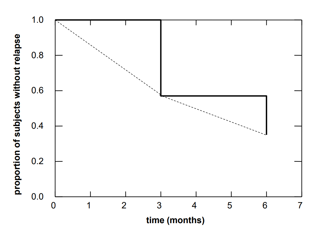
The step curve starts at a value of \(1\) and has a first drop at \(3\) months where the new value equals the observed proportion of study participants without a relapse during the first three months. It has a second drop at \(6\) months where the new value equals the estimated proportion of study participants without a relapse during the entire six month period. In reality, this curve would also decrease between the time points of 0, 3 and 6 months. Since we do not know the time points of the relapses, we cannot provide a more refined picture. At best, we could connect the lower step points linearly with each other (dashed line). However, this would only be correct if the number of study participants had been very large and time intervals between consecutive relapses had all been of the same length. If the sample had been very large and Dr. Stein had been able to observe each relapse immediately, he would have obtained an almost smooth curve with a large number of tiny steps.
Next, Dr. Stein examines the results observed in treatment group \(B\). They are summarised in the following table:
| Number | |
|---|---|
| patients in the beginning | 248 |
| had relapse within 3 months | 93 |
| had no relapse within 3 months | 155 |
| no longer observed after 3 months (among those without a relapse) | 23 |
| still observed after 3 months | 132 |
| had relapse within months 4-6 | 33 |
| had no relapse within months 4-6 | 99 |
Now Dr. Stein would like to know if the observed difference in the frequencies of relapses between the two smoking cessation programs might be explained by chance alone or not. For this, he could try to compare the frequencies of relapses between the two programs for each period separately using the Chi-squared test or Fisher's exact test (cp. chapter 12). This would certainly be a reasonable approach. However, the question would arise how the two partial results could be summarised into one result.
Since this is not quite simple, another method is used, which we will now briefly sketch. Under the null hypothesis, stating that the two cessation programs do not differ in the frequencies of relapses, these probabilities could be estimated by pooling the two groups. This would lead to the following table:
| number | |
|---|---|
| patients in the beginning | 469 |
| relapse within 3 months | 188 |
| no relapse within 3 months | 281 |
| no longer observed after 3 months (among those without a relapse) | 59 |
| still observed after 3 months | 222 |
| relapse within months 4-6 | 68 |
| no relapse within months 4-6 | 154 |
Under the null hypothesis the probability of relapsing within the first three months can be estimated at \(188/468 = 0.401\). Among the individuals without a relapse in the first three months, \(281 - 59 = 222\) are still available for the assessment after six months. \(68\) of them had a relapse. The probability of having a relapse in the second three month period can thus be estimated at \(68/222 = 0.306\). If these were the true probabilities for both cessation programs, then we would have expected the following numbers of relapses for group \(A\)
However, as in all statistical tests, we can not properly interpret the test statistic without looking at its standard error. The value of the standard error is \(6.29\) in our case. It is calculated from the standard errors of the differences between the observed and the expected relapses in the two separate time periods. The respective formula can be found in the mathematical appendix of the course. The \(t\)-value of the test statistic is \(13.9/6.29 = 2.21\). This value corresponds to the \(0.986\)-quantile of the standard normal distribution. The respective \(p\)-value is thus \(2\times(1-0.986) = 0.028\). It gives the probability with which we would have had to expect a value of the test statistic at least as different from \(0\) as the one observed, if the null hypothesis were true. In this case, the null hypothesis postulates that the two cessation programs have the same relapse probabilities in both three month periods. Since the p-value is smaller than \(0.05\), we can reject the null hypothesis at the usual \(5\%\)-level. This supports the hypothesis that the risk of having a relapse within six months is higher in program \(A\).
Would we have come to the same conclusion if we had based our calculations on the results of program \(B\)? The answer is yes. In this case, the difference between the observed and the expected number of relapses would have had the same absolute value but the opposite sign (i.e., -13.9). Moreover, the standard error would have been identical (i.e., 6.29). We would thus again have obtained a \(p\)-value of \(0.028\).
In the following example we will examine the survival of patients with metastasising colon cancer, who received two different treatments with Irinotecan (low weekly dosage vs. high three-weekly dosage), in addition to the standard treatment with Capecitabine. The assignment of the patients to the two treatments was done by randomisation [1]. The individual survival times (in weeks) are listed for both groups in the following table:
| weekly treatment (group A) | 8 19 19 29 30 35 36 37 40 44 50 50 50+ 52 55 57 59+ 60+ 62+ 64 65+ 65+ 65+ 68 68+ 68+ 68+ 71+ 72+ 72+ 74+ 75+ 76 76+ 77 84 97 100+ |
|---|---|
| three-weekly treatment (group B) | 21 35 37 37 45 46 49+ 52+ 58 60 61+ 63 64+ 65 65+ 65+ 65+ 66+ 67+ 69 69+ 71 81+ 82+ 82+ 83+ 83+ 84+ 85+ 88+ 89 89+ 93+ 93+ 101+ 107 115+ |
Improper survival times are marked with the symbol \(+\). They are from patients in whom the event of interest could not be observed. There may be various reasons for this:
In these cases, the survival time is defined as the length of the time interval during which the respective patient was observed in the study. We then speak of "censored" survival times, since the event of interest could not be observed.
There had also been censored observations in the first example. They originated from those individuals who were still non-smokers after three months but then withdrew from the study, which corresponds to case b).
However, in the present example, all censored survival times are of type a). Since patients were gradually recruited into the study, those recruited towards the end of the study could only be observed during a short time period and were likely to still be alive when the study ended. Notice, that every patient has his own clock starting at the time of inclusion into the study. Thus, the survival time of a patient who died during the study, equals the difference between the date of death and the date of inclusion. Moreover, for a patient whose death could not be observed during the study, the censored survival time equals the difference between the date when he/she was last observed alive and the date of inclusion. For simplicity, survival times are indicated in rounded weeks in the present example.
The simultaneous occurrence of censored and uncensored survival times explains why such data require special analytic methods.
|
Synopsis 15.2.1
If the occurrence of an event of interest cannot be observed in a person, then the time during which he/she was observed is used as substitute for the unobserved survival time. Such improper survival times are generally referred to as "censored" or as "event-free" survival times and the respective events as "censoring events". The simultaneous occurrence of censored and uncensored survival times requires special analytic methods. |
We will now look at the survival curves of the two groups of patients.
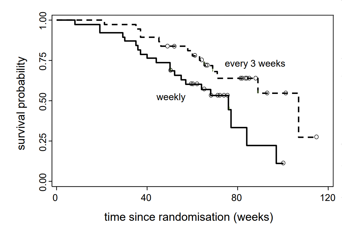
For each value \(t\) of time since inclusion (x-axis), the \(y\)-coordinate of the curve point indicates the estimated probability for patients of the respective group to survive until time \(t\). At the steps of the curve, the \(y\)-value on the lower edge counts. The tiny circles indicate censoring events. Since these are not real events, the survival curve does not have steps at these points. Nevertheless the number of individuals, who remain under onbservation or - as one also says - who are still at risk, changes. This number also decreases after censoring events. The effect of a censoring event can be seen indirectly, in that the step size at the time of the next real event increases.
The two survival curves show that, almost from the beginning, the estimated survival probabilities are higher in the group with a three-weekly administration of Irinotecan than in the group to which Irinotecan was administered on a weekly basis. Patients who had been treated with Iriontecan every three weeks thus have survived longer, on average.
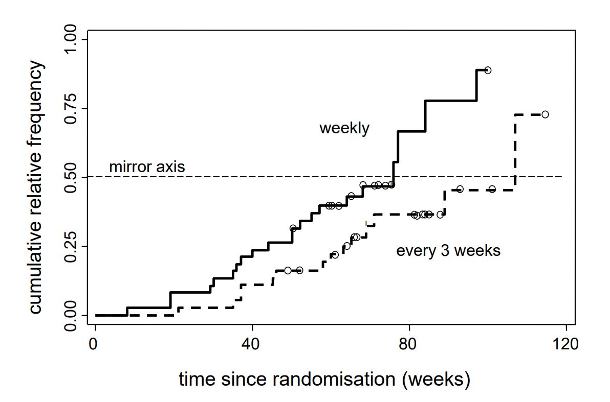
As the question above suggests, there is a direct relation between survival curves and distribution functions. If we mirror the survival function at the horizontal line with \(y = 0.5\), we get the estimated distribution of the variable survival time. The respective reflected curves are illustrated in the following figure.
By means of the example of the colon cancer patients with a three-weekly administration of Irinotecan (group B), we want to explain the construction of the survival curve based on the following table. .
| Interval | \(t_i\) (weeks) | \(n_i\) | \(d_i\) | \(z_i\) | \(n_i - d_i\) | \(p_i = \frac{n_i-d_i}{n_i}\) | \(s_i\) |
|---|---|---|---|---|---|---|---|
| 1 | 21 | 37 | 1 | 0 | 36 | \(36/37 = 0.973\) | 0.973 |
| 2 | 35 | 36 | 1 | 0 | 35 | \(35/36 = 0.972\) | 0.946 |
| 3 | 37 | 35 | 2 | 0 | 33 | \(33/35 = 0.943\) | 0.892 |
| 4 | 45 | 33 | 1 | 0 | 32 | \(32/33 = 0.970\) | 0.865 |
| 5 | 46 | 32 | 1 | 0 | 31 | \(31/32 = 0.969\) | 0.838 |
| 6 | 49 | 31 | 0 | 1 | 31 | \(31/31 = 1.000\) | 0.838 |
| 7 | 52 | 30 | 0 | 1 | 30 | \(30/30 = 1.000\) | 0.838 |
| 8 | 58 | 29 | 1 | 0 | 28 | \(28/29 = 0.966\) | 0.809 |
| 9 | 60 | 28 | 1 | 0 | 27 | \(27/28 = 0.964\) | 0.780 |
| 10 | 61 | 27 | 0 | 1 | 27 | \(27/27 = 1.000\) | 0.780 |
| 11 | 63 | 26 | 1 | 0 | 25 | \(25/26 = 0.962\) | 0.750 |
| 12 | 64 | 25 | 0 | 1 | 25 | \(25/25 = 1.000\) | 0.750 |
| 13 | 65 | 24 | 1 | 3 | 23 | \(23/24 = 0.958\) | 0.719 |
| 14 | 66 | 20 | 0 | 1 | 20 | \(20/20 = 1.000\) | 0.719 |
| 15 | 67 | 19 | 0 | 1 | 19 | \(19/19 = 1.000\) | 0.719 |
| 16 | 69 | 18 | 1 | 1 | 17 | \(17/18 = 0.944\) | 0.679 |
| 17 | 71 | 16 | 1 | 0 | 15 | \(15/16 = 0.938\) | 0.636 |
| 18 | 81 | 15 | 0 | 1 | 15 | \(15/15 = 1.000\) | 0.636 |
| 19 | 82 | 14 | 0 | 2 | 14 | \(14/14 = 1.000\) | 0.636 |
| 20 | 83 | 12 | 0 | 2 | 12 | \(12/12 = 1.000\) | 0.636 |
| 21 | 84 | 10 | 0 | 1 | 10 | \(10/10 = 1.000\) | 0.636 |
| 22 | 85 | 9 | 0 | 1 | 9 | \(9/9 = 1.000\) | 0.636 |
| 23 | 88 | 8 | 0 | 1 | 8 | \(8/8 = 1.000\) | 0.636 |
| 24 | 89 | 7 | 1 | 1 | 6 | \(6/7 = 0.857\) | 0.546 |
| 25 | 93 | 5 | 0 | 2 | 5 | \(5/5 = 1.000\) | 0.546 |
| 26 | 101 | 3 | 0 | 1 | 3 | \(3/3 = 1.000\) | 0.546 |
| 27 | 107 | 2 | 1 | 0 | 1 | \(1/2 = 0.500\) | 0.273 |
| 28 | 115 | 1 | 0 | 1 | 1 | \(1/1 = 1.000\) | 0.273 |
We have to proceed step by step, as we already did in the introductory example of the smoking cessation programs. Each new event time point \(t_i\) initiates a new interval. The \(i\)-th time interval starts at \(t_{i-1}\) and ends at \(t_i\). Thus, we must have \(t_0 = 0\). Sometimes, the number of events at a given time point \(t_i\) is larger than \(1\). This is mainly because survival times were recorded in weeks. Had they been recorded in days, most if not all events would have occurred at different times.
\(n_i\) stands for the number of patients still under observation at the beginning of the \(i\)-th time interval. These are the patients who did not have an event prior to \(t_i\) and are still under observation after \(t_i\).
\(d_i\) stands for the number of patients having survived \(t_{i-1}\) but not \(t_i\). The probability of surviving the \(i\)-th time interval after having been alive and under observation immediately after time \(t_{i-1}\) is estimated by \[ p_i = \frac{n_i-d_i}{n_i} .\] The number of patients \(n_{i+1}\) still under observation after time point \(t_i\) equals \[n_{i+1} = n_i - d_i - z_i \,,\] where \(z_i\) stands for the number of patients with a censoring event at time point \(t_i\).
By \(s_i\) we denote the estimated probability of surviving time \(t_i\). In analogy to the first example, the probability of surviving \(t_{i+1}\) is estimated as follows \[s_{i+1} = s_i \times p_{i+1} \, ,\] starting with \[s_1 = p_1 .\] From this it follows that \(s_2 = p_1 \times p_2\), \(s_3 = p_1 \times p_2 \times p_3 \) and \(s_i = p_1 \times p_2 \times ...\times p_i .\) As an example, the value of \(s_7\), i.e., the estimated probability of surviving \(52\) weeks is \(0.973 \times 0.972 \times 0.943 \times 0.970 \times 0.969 \times 1 \times 1 = 0.838\).
When constructing survival curves, we implicitly assume that individuals with censored observations would have had a similar further follow-up history as those who remained under observation. However, this assumption must often be questioned. Often, individuals who leave the study early, have a worse prognosis. Therefore one might also consider an early withdrawal from the study as negative outcome and then test with a two-by-two table, if the frequency of negative outcomes differs significantly between the groups or not. This is sometimes done as "worst case"-analysis. Fortunately, there is no need for such concerns in the present example, as all censoring events occurred at the end of the study.
With the applet "Kaplan-Meier survival curve" you can define true and censoring events along the survival time axis, starting from an initial sample whose size you can specify. With each new event, the survival curve changes. By clicking below the survival curve, you set a new true event (i.e., with an uncensored survival time) at the respective time point, and by clicking above the survival curve you define a censoring event. The survival curve will reach \(0\) after you have set as many events as there were subjects in the initial sample.
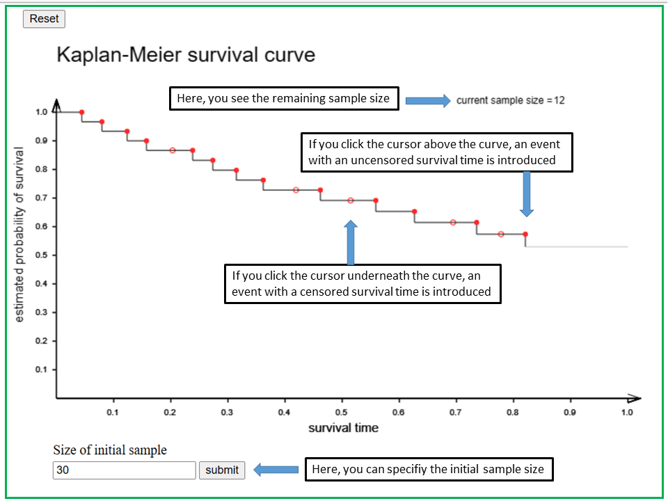
With the applet "Kaplan-Meier survival curve" you can define uncensored and censored events along a time axis, starting from an initial sample whose size you can specify at the beginnung in the box at the bottom. If you don't specify the sample size, it is assumed to be 20.
At the beginning, the survival curve is a horizontal line with y-coordinate = 1 (corresponding to a survival probability of 1). If you click the cursor below the survival curve, you set a new true event with an uncensored survival time at the x-coordinate of the cursor. By clicking above the survival curve you define a censored survival time.
Each new event will change the shape of the survival curve. The number of subjects who are still at risk is indicated in the upper left part of the panel as "current sample size". The current sample size and the survival curve will eventually drop to 0 after you have set as many events as there were subjects in the initial sample.
How does the shape of the survival curve change if you set a new true event with an uncensored survival time, and how does it change if you set an event with a censored survival time?
After having examined the survival curves of the two groups of colon cancer patients, we are interested whether or not the observed differences between the two survival curves might be explained by chance alone or whether there is evidence for a different survival under the two treatments.
To answer this question, we need a statistical test which can assess the differences between two curves. This is a more complex task than just comparing two simple measures (e.g., two sample means or proportions). In the introductory example, we already encountered the basic idea of such a comparison. Although we now have a much larger number of time intervals, the procedure of calculating the test statistic is the same. To illustrate this, we will take a look at the beginning of the table underlying the calculations.
| Event in group | Time point (weeks) | \(n_A\) | \(d_A\) | \(n_B\) | \(d_B\) | \(n\) | \(d\) | \(q = d/n\) | |
|---|---|---|---|---|---|---|---|---|---|
| A | 8 | 38 | 1 | 37 | 0 | 75 | 1 | \(1/75 = 0.0133\) | |
| A | 19 | 37 | 2 | 37 | 0 | 74 | 2 | \(2/74 = 0.0270\) | |
| B | 21 | 35 | 0 | 37 | 1 | 72 | 1 | \(1/72 = 0.0139\) | |
| A | 29 | 35 | 1 | 36 | 0 | 71 | 1 | \(1/71 = 0.0141\) | |
| A | 30 | 34 | 1 | 36 | 0 | 70 | 1 | \(1/70 = 0.0143\) | |
| A,B | 35 | 33 | 1 | 36 | 1 | 69 | 2 | \(2/69 = 0.0290\) | |
| . | . | . | . | . | . | . | . | ... |
This table was generated by merging the chronological event lists of both groups. The symbols \(n_A\) and \(n_B\) denote the numbers of individuals in groups \(A\) and \(B\) who were at risk prior to the occurrence of the respective event. The symbols \(d_A\) and \(d_B\) denote the numbers of deaths in the two groups recorded at the end of the respective time interval, and the symbols \(n\) and \(d\) represent the respective numbers of the two groups combined. Hence \(n = n_A + n_B\) and \(d = d_A + d_B\) holds.
In the pooled sample, the observed proportion of patients with an event is \(q = d/n\). In this case, the null hypothesis states that, in each time interval, the probability of having an event is the same for both groups. What would this imply for the individual probability of experiencing the event of interest in the \(i\)-th time interval conditional on having survived without the event before? Under the null hypothesis, we would postulate the same event probability of \(0.0133\) in the first time interval for group \(A\) and group \(B\). In group \(A\), we would therefore expect \(38 \times 0.0133 = 0.51\) cases in the first interval, and in group \(B\) these would be \(37 \times 0.0133 = 0.49\) cases. The sum of the two expected values equals the number of observed cases in the respective interval. For the second interval, we would estimate an event probability of \(2/74 = 0.0270\) in both groups and thus expect \(37 \times 0.027 = 1.0\) cases in group \(A\), with \(37\) individuals at risk at the beginning of this interval. In the third interval, we would expect \(35 \times 0.0139 = 0.49\) cases in group \(A\).
If we continued like this, we would get \(0.51 + 1.0 + 0.49 + 0.49 + 0.49 + 0.96 = 3.94\) expected cases in the first six time intervals for group \(A\). This contrasts with the \(1 + 2 + 0 + 1 + 1 + 1 = 6\) observed cases.
As in the introductory example of smoking cessation, we consider the difference between the number of observed and the number of expected cases. For the first six time intervals it equals \(6 - 3.94 = 2.06\). If one sums up the observed and the expected numbers of cases across all time intervals and then takes the difference between the two sums, one obtains the test statistic of the so-called "log rank test".
In our example we can find by counting that the total number of observed deaths in group \(A\) is \(21\). On the other hand, we would obtain a total of \(14.73\) expected events when completing the stepwise calculations. The difference between these two numbers equals \(21-14.73 = 6.27\). In the next step, we must divide this difference by its standard error \(2.85\) (this value can be calculated using the formulas in the Mathematical Appendix). Therefore, the \(t\)-value equals \( 6.27/2.85 = 2.2 \). By squaring the \(t\)-value, we get the Chi-squared value of the log rank test, \(4.84\).
Under the null hypothesis, the distribution of this test statistic comes close to a Chi-squared distribution with \(1\) degree of freedom, provided that the group sizes are not too small. The value of \(4.84\) equals the \(97\)-th percentile of the Chi-squared distribution with \(1\) degree of freedom. Therefore the \(p\)-value equals \(0.03\). The difference between the two survival curves is thus statistically significant at the \(5\%\)-level. However, as the nature of the study was exploratory (i.e. no prior hypotheses were formulated), no formal inference should be made from this result.
Remark: To be able to conduct the above calculations, we must know when the individual events occurred, in which group they occurred and whether they were true or censoring events. Therefore, a data table used for survival analysis must include at least three columns (variables):
The log rank test works well, if one group has the higher estimated survival probabilities than the other one across the entire observation period (i.e., if the survival curves do not intersect after \(t = 0\)). It works particularly well if the relative difference between the \(y\)-values of the two survival curves increases with time.
A completely different situation is given if the two survival curves intersect each other at some point and the curve which decreased more steeply in the beginning continues at a higher level beyond the point of intersection. Such an example is given in the figure below.
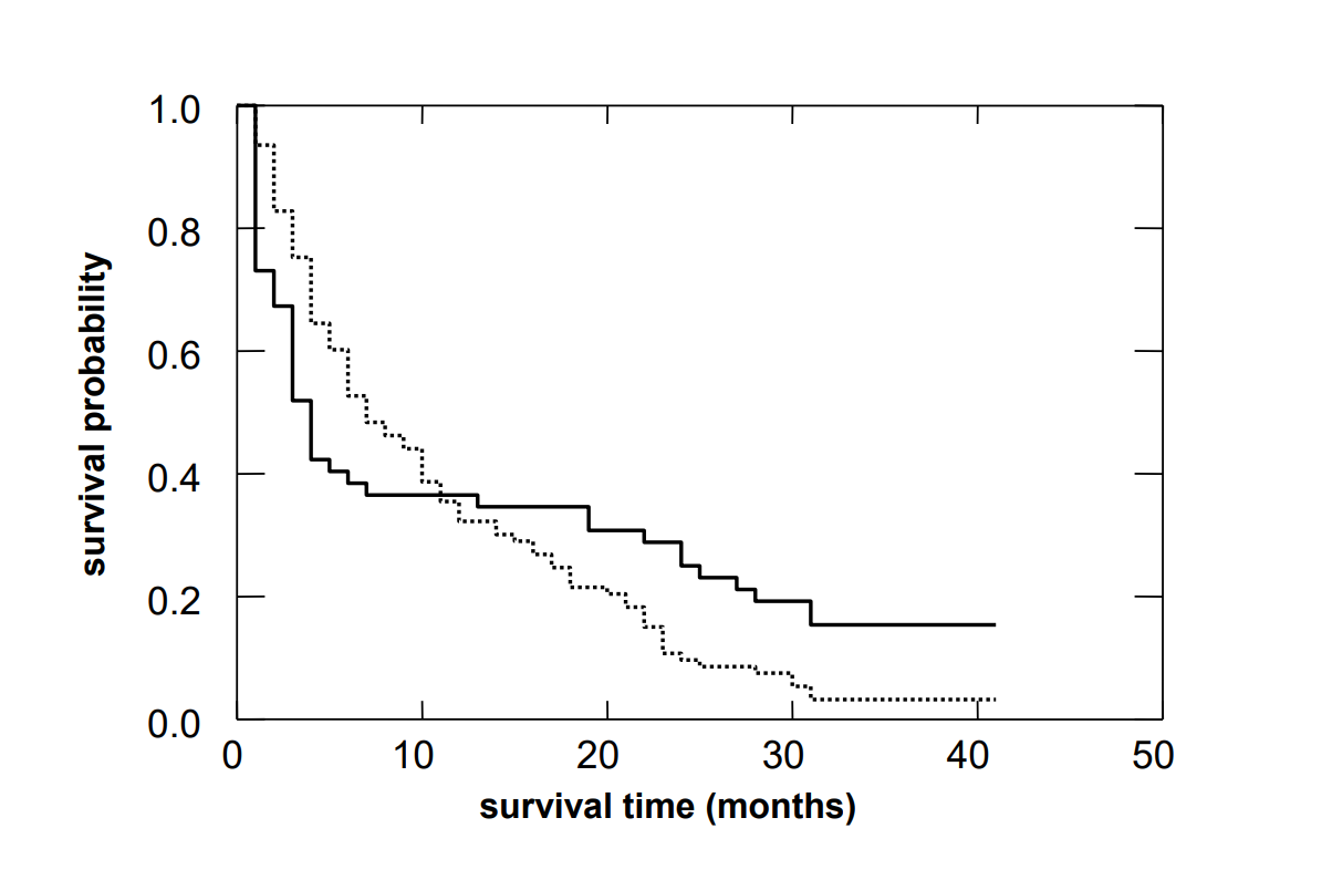
The log rank test is blind to such differences. Results of the log rank test should thus not be interpreted without looking at the survival curves. A situation, as illustrated in the figure above, can occur if one of the two interventions is associated with an increased risk of mortality in the beginning but improves the long term outcome of patients who survive the critical initial phase. In such cases, it makes sense to perform separate survival analyses for the first phase after the intervention and for the further course after the initial phase.
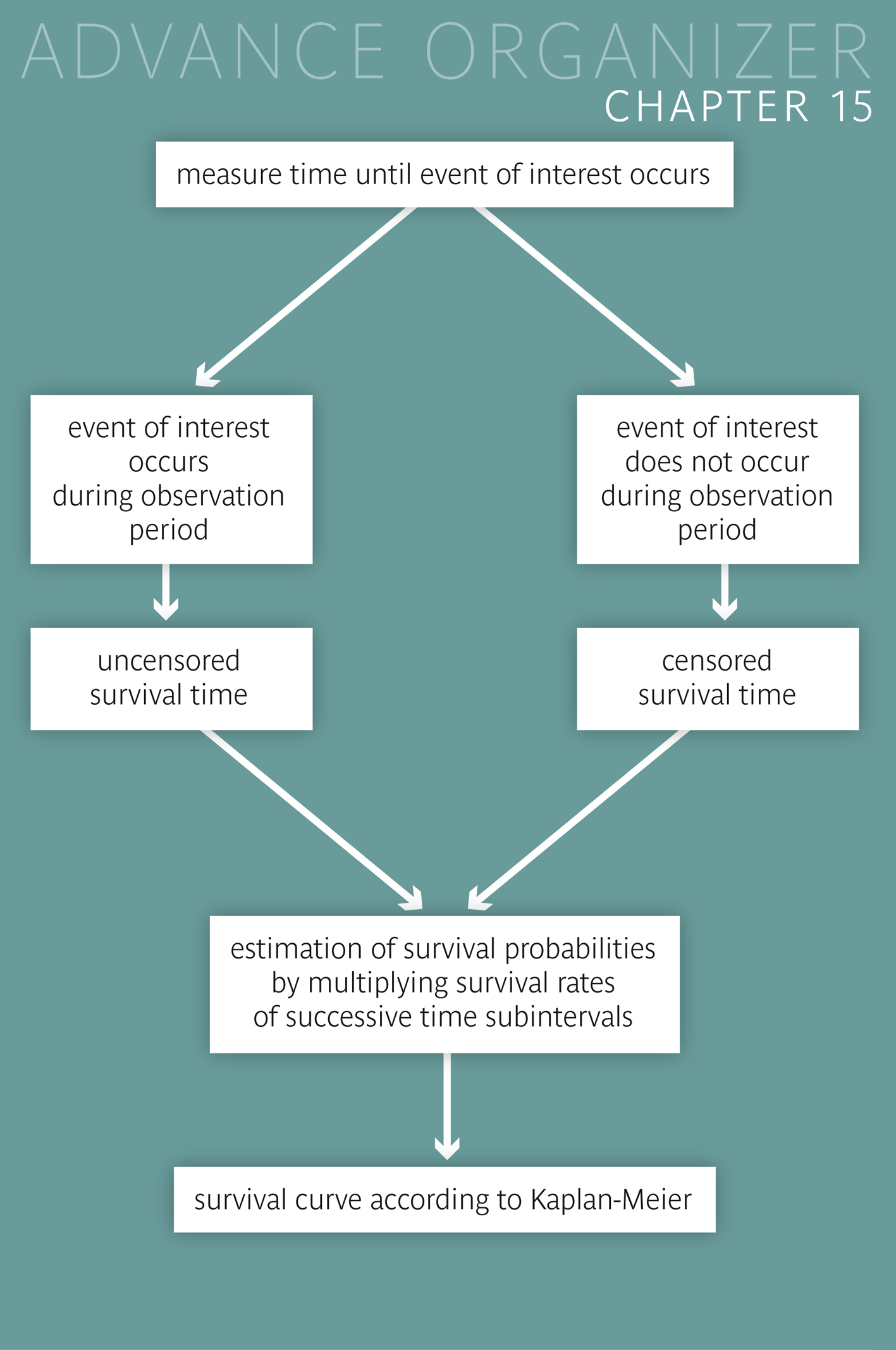
When working with patients, we are often interested in the time until a specific event (death, life threatening problem, relapse, remission, etc.) occurs. If this event occurs before the end of the observation period, this time can be determined exactly. Otherwise, the time during which the person was observed has to be recorded instead. In the first case we speak of uncensored and in the latter case of censored survival times.
The existence of censored survival times complicates the estimation of survival probabilities. Since a direct calculation of survival rates is only possible for time intervals without censored observations, the whole observation period has to be divided into separate time intervals, so that true and censoring events always define the beginning of a new time interval. For each of these time intervals, the survival probability is estimated by the ratio \( (n - d)/n \) where \(n\) denotes the number of individuals at risk at the beginning of the interval and \(d\) denotes the number of true events in the interval. The probability of surviving a specific follow-up time point without the event of interest is estimated by the product of the estimated survival probabilities in the intervals preceding the time point.
For the statistical evaluation of the differences between two survival curves, the log rank test is commonly used. However, for this test to work properly, the two survival curves should not intersect.
[1] M.M Borner et al. (2005),
A randomized phase II trial of capecitabine and two different
schedules of Irinotecan in first-line treatment of metastatic colorectal
cancer: efficacy, quality of life and toxicity
Annals of Oncology, 16(2), pp 282-88.