
|
The last two chapters were devoted to statistical tests for quantitative variables. However, scientific questions often also or even exclusively involve categorical variables and thus ask for frequency comparisons. Two or more independent samples with categorical data are compared with the "chi-square-test" or "Fisher's exact test". The comparison of paired binary data is treated with the McNemar test. |
|
Educational objectives
After having worked through this chapter you will be able to choose the suitable test for the comparison of two or more samples with categorical data and you can interpret the test results correctly. Key words: frequency tables, general two-way tables, Chi-squared test, Fisher's exact test, McNemar's testPrevious knowledge: mean value, median (chap. 3), normal distribution (chap. 6), statistical hypotheses, statistical hypothesis testing, significance level, p-value (chap. 9) Central questions: How can we judge whether the distribution of a categorical variable differs significantly between different comparison groups? |
To start with we will examine an example of a two-by-two table. In a study by Zanghieri et al. (1990) (cf. [1], page 553), \(132\) patients with colorectal cancer were examined to find out whether there is an association between the histological disease type ("diffuse" or "intestinal") and a colorectal cancer disease in first-degree relatives ("familyanamnesis positive" vs. "family anamnesis negative"). The data are listed in table 12.1.
| Diffuse | Intestinal | Total | |
|---|---|---|---|
| family anamnesis + | 13 | 12 | 25 |
| family anamnesis - | 35 | 72 | 107 |
| Total | 48 | 84 | 132 |
In this case, we have following two complementary hypotheses \[ H_A : \text{There is an association between the two variables}\] and \[ H_0 : \text{The two variables are independent}\]
By "association" we mean that the two variables are not independent, i.e., that the distribution of each of the two variables varies across the categories of the other variable.
Under \(H_0\), both types of patients would have the same probability of a positive family anamnesis. The best estimate of this probability we can obtain with the available data is the ratio "number of patients with a positive family anamnesis" / "total number of patients". This ratio equais \( \frac{25}{132} = 0.189 \). Under \(H_0\) and if this were the true probability in the underlying population, we would on average expect \( 48 \times \frac{25}{132} = 9.091 \) patients with a positive family history in repeated random samples of \(48\) patients with the disease type "diffuse". Likewise, we would on average expect \( 84 \times \frac{25}{132} = 15.909 \) patients with a positive family history in repeated random samples of \(84\) patients with disease type "intestinal".
Complementary to these numbers, we would, on average, expect \( 48 - 9.091 = 38.909 \) patients with a negative family history among \(48\) patients with the disease type "diffuse" and \( 84 - 15.909 = 68.091 \) with a negative family history among \(84\) patients with the disease type "intestinal". All of these expected frequencies are higher than 5.
Under the condition that the expected number of people of each cell of the table is at least \(5\) under \( H_0 \), we can use the \(\chi^{2}\)-test (Chi-squared test) to \(H_A\).
In our example the condition for the application of the \(\chi^{2}\)-test is thus fulfilled.
The test statistic \(\chi^{2}\) is calculated based on a comparison of the observed and the expected frequencies in the cells of the two-by-two table. The differences between the observed and the expected frequencies are listed in table 12.2.
| Diffuse | Intestinal | Total | |
|---|---|---|---|
| family anamnesis + | 13 - 9.091 - 3.909 | 12 - 15.909 = -3.909 | 0 |
| family anamnesis - | 35 - 38.909 = -3.909 | 72 - 68.091 = 3.909 | 0 |
| Total | 0 | 0 | 0 |
All four differences have the same absolute value but different signs. To get rid of the signs, the differences are squared. Intuitively, one might think that the sum of the squared differences would be a good test statistic, because it measures how different the observed frequencies are from the expected ones under \(H_0\). However, even under \(H_0\), the difference between an observed and an expected frequency tends to increase with the size of the expected frequency, as we have seen with the Poisson distribution in chapter 7. The "statistical" comparability of the squared differences can be achieved upon dividing them by the respective expected frequencies. This provides us with the following standardized squared differences for our example \( 3.9092/9.091 = 1.681 \) , \( 3.9092/38.909 = 0.393 \), \( 3.9092/15.909 = 0.960 \) and \( 3.9092/68.091 = 0.224 \).
The test statistic of the \(\chi^{2}\)-test is now defined as the sum of these standardised squared differences. It gets the value \(3.258\) in our example. Under \(H_0\), the probability of obsering a \(\chi^{2}\)-value larger than a positive number \(c\) decreases with \(c\). This probability equals \(0.05\) if \(c = 3.84\). Therefore, \(c = 3.84\) is the critical limit for the \(\chi^{2}\)-test of a two-by-two table if we assume a significance level \( \alpha = 0.05 \).
The null hapothesis \( H_0 \) can also be formulated in terms of equations for the joint probabilities of independent events (cf. chapter 5): \[ P(\text{"fam.anam. +" and "intestinal"}) = P(\text{"fam.anam. +"}) \times P( \text{"intestinal"}) \] \[ P(\text{"fam.anam. +" and "diffuse"}) = P(\text{"fam.anam. +"}) \times P(\text{"diffuse"}) \] \[ P(\text{"fam.anam. -" and "intestinal"}) = P(\text{"fam.anam. -"}) \times P(\text{"intestinal"}) \] \[ P(\text{"fam.anam. -" and "diffuse"}) = P(\text{"fam.anam. -"}) \times P( \text{"diffuse"} ) \]
In the next example, we will analyse a 3-by-4 table.
In a study on Hodgkin's disease by Hancock et al. [2], \(538\) patients were divided into the \(4\) groups \(LP\) (lymphocyte predominant), \(NS\) (nodular sclerosing), \(MC\) (mixed cellularity) and \(LD\) (lymphocyte depletion), based on the histology of their cancer. A second classification of the patients was done based on their response to treatment after three months (with categories "positive", "partial" and "none").
Is there an association between the histological type of disease and therapy response? The results of this study are listed in table 12.3.
| Response | ||||
|---|---|---|---|---|
| Histological type | positive | partial | none | Total |
| LP | 74 | 18 | 12 | 104 |
| NS | 68 | 16 | 12 | 96 |
| MC | 154 | 54 | 58 | 266 |
| LD | 18 | 10 | 44 | 72 |
| Total | 314 | 98 | 126 | 538 |
We are interested in the hypotheses \[H_A : \text{therapy response depends on the histological type of disease.} \] vs. \[H_0 : \text{therapy response does not depend on the histological type of disease.} \] If the average cell frequencies expected under \(H_0\) are all \(\geq 5\), we can use the \(\chi^{2}\)-test in this case as well. We verify that the condition is met by looking at the cell belonging to the disease type category with the lowest frequency (i.e., \(NS\) with \(n = 96\)) and the response category with the lowest frequency (i.e. "partial" with \(n = 98\)), and calculating the expected frequency for the respective cell as \(\frac{96 \times 98}{538} = 17.5\). As all other cells have higher expected frequencies under \(H_0\), the condition is satisfied.
As in the case of the two-by-two table we first square the difference between the observed and the expected frequency for each of the \(12\) cells and then divide the result by the expected frequency. Finally, we add these standardised squared differences. In the present example, we obtain a value of \(74.89\) for the \(\chi^{2}\)-statistic.
Because of the larger number of cells, the critical limit at the significance level of \(\alpha=0.05\) is larger than \(3.84\) in this example. Under the the null hypothesis, the \(\chi^{2}\)-test statistic follows a \(\chi^{2}\)-distribution with \( (3-1)\times(4-1) = 6\) degrees of freedom. (The number of degrees of freedom is calculated as the product \( \text{(number of rows - 1)} \times \text{(number of columns - 1)}\).
In Excel, one can get the critical limit for this test as the \(95\)-th percentile of the \(\chi^{2}\)-distribution with \(6\) degrees of freedom, by evaluating \(CHISQ.INV(0.95;6)\). It provides a value of \(12.59\). The value of our test statistic, \(75.89\), is much larger. In fact, the \(p\)-value of our result can be obtained in Excel by evaluating \(CHISQ.DIST.RT(75.89;6)\). It is extremely small and even much smaller than \(0.001\). The observed association between the two variables is thus highly significant (\(p\)-values \(\lt 0.001\) are often referred to "highly significant").
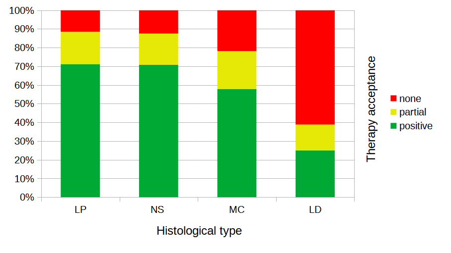
The differences in the distribution of therapy response across the different histological categories is illustrated in the following stacked bar chart. While the response was high in the categories \(LP\) and \(NS\), it was lower in category \(MC\) and particularly low in category \(LD\).
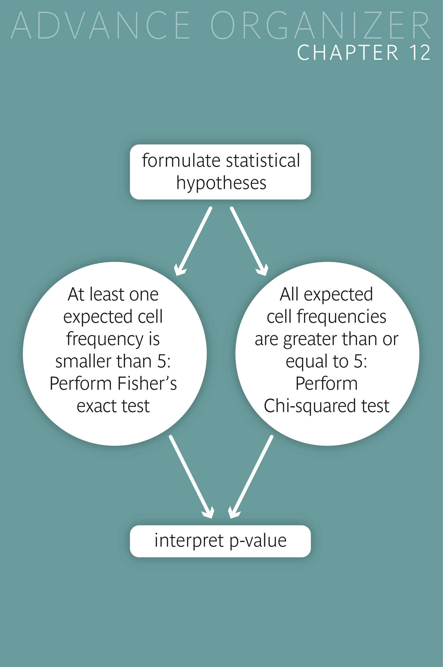
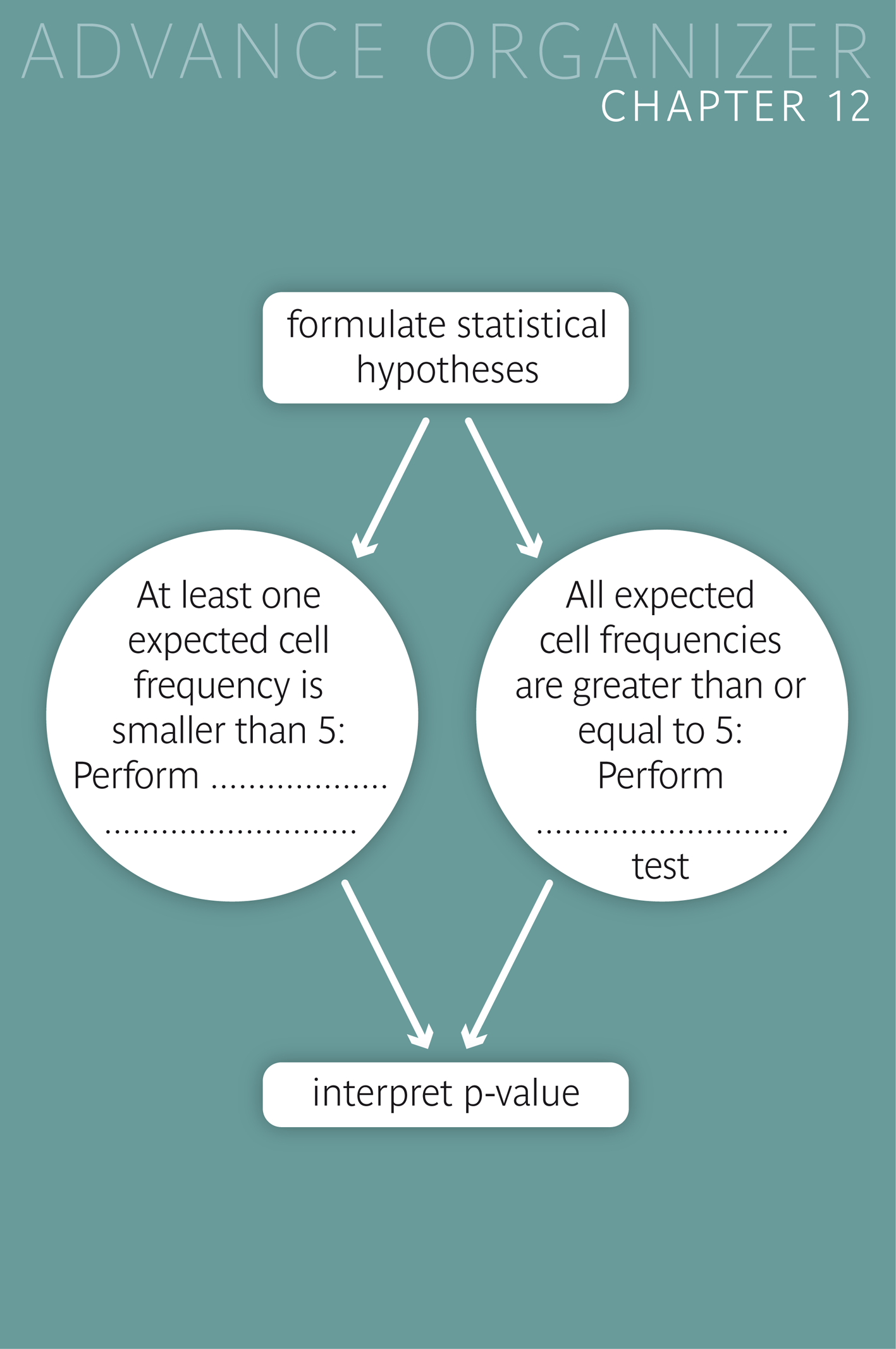
If some expected cell frequencies are smaller than \(5\) under \(H_0\), the validity of the \(\chi^{2}\)-test may be violated. Most statistics programs will then show the results nevertheless, but they will give out a warning.
Alternatively, Fisher's exact test can be used. This test provides exact \(p\)-values and represents the ideal choice for small sample sizes. With this test, the probabilities of the various possible frequency tables with the same row and column totals as in the observed table are calculated under the null hypothesis using combinatorics. The probabilities of frequency tables which are less likely than the observed one are added up to obtain the \(p\)-value of the observed table.
|
Synopsis 12.1.1
The Chi-squared test and Fisher's exact test serve to assess whether the association of two variables in a two-way table is statistically significant or not. Fisher's exact test is ideal for small sample sizes. This test should be applied if at least one of the expected cell frequencies lies under \(5\). In the case of a general two-way table the Chi-squared test should be applied whenever possible due to the computational effort of the exact test. If individual expected cell frequencies are smaller than \(5\), it is advisable to simplify the table by collapsing small categories, which reduces the number of rows and/or columns of the table. |
Since it was already known that the frequency of genotype \(G\) is elevated in persons with disease \(D\), a new study examined if the frequency of genotype \(G\) might additionally depend on the severity of the diseae \(D\). A random sample of \(116\) patients with disease \(D\) provided the following results
| Genotype \(G\) | Other genotype | Total | |
|---|---|---|---|
| severe type of \(D\) | 9 | 7 | 16 |
| less severe type of \(D\) | 27 | 73 | 100 |
| Total | 36 | 80 | 116 |
With the applet "Chi-squared test for 2x2 table" you can modify the cell frequencies of a two-by-two table by moving lines (as in the Bayes-applet of chapter 5). On the right hand side, the three consecutive tables used to calculate the Chi-squared statistic are displayed and continually updated while you change the table.
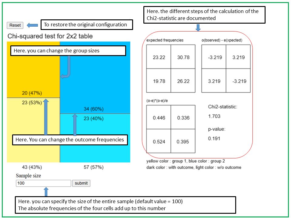
In the applet "Chi2-test", you can define and modify a two-by-two table graphically and observe how the different intermediate results of the calculation of the Chi2-statistic change. The two-by-two table is represented as a square consisting of four rectangles. The areas of the rectangles represent the cell frequencies. As soon as you enter a sample size n in the entry field at the bottom, absolute and relative frequencies are displayed in the four rectangles. These numbers are roughly proportional to the areas of the rectangles.
With the vertical line you define the distribution of the first binary variable X1 which defines the two groups. The yellow area to the left of the vertical line represents the probability P(X1=1) and the blue area to the right the probability P(X1=0). In the initial setting, the vertical line cuts the square in half, which corresponds to a situation with P(X1=1) = P(X1=0) = 0.5.
The second variable X2 might indicate the presence (X2=1) and absence (X2=0) of a specific characteristic or outcome of interest.
With the left horizontal line you can define the conditional probabilities P(X2=1|X1=1) (dark yellow area) and P(X2=0|X1=1) (light yellow area), and with the right horizontal line the conditional probabilities
P(X2=1|X1=0) (dark blue area) and P(X2=0|X1=0) (light blue area). If the two lines are at different levels, then the variables are dependent (associated), otherwise they are independent. If the two horizontal lines are at the same level, the observed frequencies and those expected under the null hypothesis (of no association between X1 and X2) are identical and the Chi2-statistic equals 0. The larger the difference between the horizontal and the vertical line, the larger the Chi2-statistic and the lower the p-value.
The horizontal and vertical lines jump while you move lines and do not move smoothly. This is because the number of tables with a given total frequency n is finite.
The Chi2-statistic and the p-value depend on the positions of the vertical and horizontal lines, but also on the sample size n. Observe what happens with the Chi2-statistic and the p-value if you leave the lines unchanged but modify the sample size. After this, you keep the sample size fixed and observe what happens when you move the vertical line while leaving the horizontal lines unchanged. Finally, you keep the sample size and the vertical line fixed while moving the horizontal lines.
If the validity condition of the Chi-squared test is violated (i.e., if one or more of the expected frequencies are smaller than 5), the respective frequencies appear in red color.
In a study by Roth et al. (1975) (cf. [3], page 272) each person was applied the potential irritant \(DNCB\) on the skin of one randomly selected arm and the potential irritant croton oil on the skin of the other arm. For each arm it was recorded whether there was a skin reaction or not. The null hypothesis was that the probability of a skin reaction does not depend on the type of irritant.
This is an example with paired data resembling the one of the cornea diameters of the sick and the healty eyes in glaucoma patients of chapter 10. However, in this case, the variables compared are binary and not numerical.
Since we are dealing with paired observations, the Chi-squared test can not be used in this case. The classical procedure to compare relative frequencies between paired samples is McNemar's test. It is a special case of the sign test.
If "irritation" is coded as \(1\) and "absence of irritation" as \(0\), then we have four possible outcomes: (DNCB: 1, Croton oil: 1), (DNCB: 1, Croton oil: 0), (DNCB: 0, Croton oil: 1) and (DNCB: 0, Croton oil: 0). The respective pairwise differences are 0, 1, -1 and 0, respectively. As outcomes with a zero difference are ignored in the sign test, only the frequencies of (DNCB: 1, Croton oil: 0) and (DNCB: 0, Croton oil: 1) will be considered and compared. They are given in the upper right and the lower left cell of the following two-by-two table.
| Croton oil | ||||
|---|---|---|---|---|
| Irritation | No irritation | Total | ||
| DNCB | irritation | 81 | 48 | 129 |
| no irritation | 23 | 21 | 44 | |
| Total | 104 | 69 | 173 | |
McNemar's test only compares the frequencies \(48\) and \(23\). Under the null hypothesis, we would expect that the two frequencies only differ by chance. More precisely, we can say that the two frequencies would have to originate from a binomial distribution with \(n = 48 + 23 = 71\) and probability \(\pi = 0.5\). The denominator \(n\) is given by the number of "discordant" pairs (i.e., observations in which the two paired values differ),
We know from chapter 7, that these values would then have to lie in the interval \[ [0.5 \times 71 - 2 \times \sqrt{71\times0.5\times0.5}, \, 0.5 \times 71 + 2 \times \sqrt{71\times0.5\times0.5} ] \] \[ = [35.5 - 8.43, 35.5 + 8.43] = [27.07, 43.93] \] with a probability of approx. \(95\%\).
However our values are not contained in this interval. Under the null hypothesis, the probability of observing a difference of the magnitude observed would thus be smaller than \(0.05\). At a significance level of \(\alpha=0.05\), the null hypothesis of equal irritation probabilities must therefore be rejected.
With a statistics program, the \(p\)-value of our result can be calculated exactly using the binomial distribution. It equals \(0.0041\). An approximate \(p\)-value can be calculated based on \( z = \frac{48 - 35.5}{0.5\times\sqrt{71}} = 2.97 \), which is the \(99.85\)-th percentile of the standard normal distribution. In this way, we would estimate the \(p\)-value to be approximately \(2\times(1 - 0.9985) = 0.003\). (You can obtain the value of the probability \(P(Z \lt 2.97)\) by evaluating \(NORM.VERT(2.97;0;1;1)\) in Excel).
|
Synopsis 12.2.1
McNemar's test is suitable for the comparison of the frequencies of two paired binary variables. |
If the question is whether two categorical variables are associated (dependent), respectively whether the frequency distribution of one of the variables varies across the categories of the other variable, the \(\chi^{2}\)-test is used.
However, this test may only be applied if the expected frequencies of the individual cells are at least \(5\) under the independence hypothesis (\( = H_0\)). Otherwise Fisher's exact test must be applied.
If the frequencies of two paired binary variables are to be compared, McNemar's test must be used. It only compares the frequencies of discordant pairs (i.e., of pairs with different values of the two variables).
[1] W.W. Daniel, (1995)
Biostatistics
John Wiley and Sons Inc.
[2] B.W. Hancock et al. (1979)
Hodgkin's disease in Sheffield (1971-76) (with computer analysis of variables)
Clinical Oncology, 5, 283-97
Data were copied from p. 60 of
[2] D.J. Hand, F. Daly, A.D. Lunn, K.J. McConway, E. Ostrowski
Handbook of Small Data Sets
Chapman and Hall, London, 1994
[3] J.A. Roth, F.R. Eilber, J.A. Nizze, D.L. Morton (1975)
Lack of correlation between skin reactivity to dinitrochlorobenzene and croton oil in patients with cancer
New England Journal of Medicine; 293: 388-9.