|
As a general rule, nothing should be left to chance. However, in empirical sciences there are standard situations, in which the contrary applies. Work through the following sections and convince yourself of this statement. |
|
Educational objectives
You can explain why samples should be drawn randomly. You can explain the terms "bias", "unbiased estimation" and "representative sample". You are familiar with the principle of randomisation and you can name concrete examples. Key words: simple random sample, stratified random samples, survey design, sample statistic, population parameter, bias, unbiased estimation method, representative sample, randomisation. Previous knowledge: population (chap. 1), sample (chap. 1), mean value (chap. 3), standard deviation (chap. 3) Central questions: How can we make valid statements with the help of chance? What does it mean to make "valid statements"? Why do we have to design a survey? |
Chance (or randomness) plays a central role in the conduct of surveys and experiments. Since we want to draw conclusions from a sample to the population from which it was drawn, the selection of elements into the sample should be done randomly. This is the only way to guarantee that the sample provides a picture of the reality at the population level which is not systematically flawed but only shows some random deviations. The easiest way to achieve this is by giving each element of the population the same chance of being selected into the sample.
|
Definition 4.1.1
If each element of a population has the same chance to be selected into the sample, then the sample is called a simple random sample. |
Randomness is also used if one wants to compare the effects of different treatments for a specific disease. In this case, individual patients with the respective disease are randomly allocated to the different treatments, a process referred to as "randomisation". This is the only way to guarantee that differences between the treatments observed after some time are only due to the treatments themselves or to chance.
Our medical practitioner, Dr. Frank N. Stein, attends to a random selection of chemical company employees. He was allocated \(18\) female and \(103\) male employees aged between \(29\) and \(76\) years. According to his mandate, he recorded variables such as weight and blood sugar for all of these patients. In his medical practice, Dr. Frank N. Stein also attends to approximately \(400\) other patients in the same range of age. About half of these patients are women. One evening the talks with his cousin, Dr. Stefan Frank, about diet, health and overweight. He tells him that the mean level of cholesterol in "his" chemical company employees equals \(224 mg/dl\) and that the mean weight equals \(74.2 kg\). He bases his subsequent reasoning on the following (debatable) assumptions
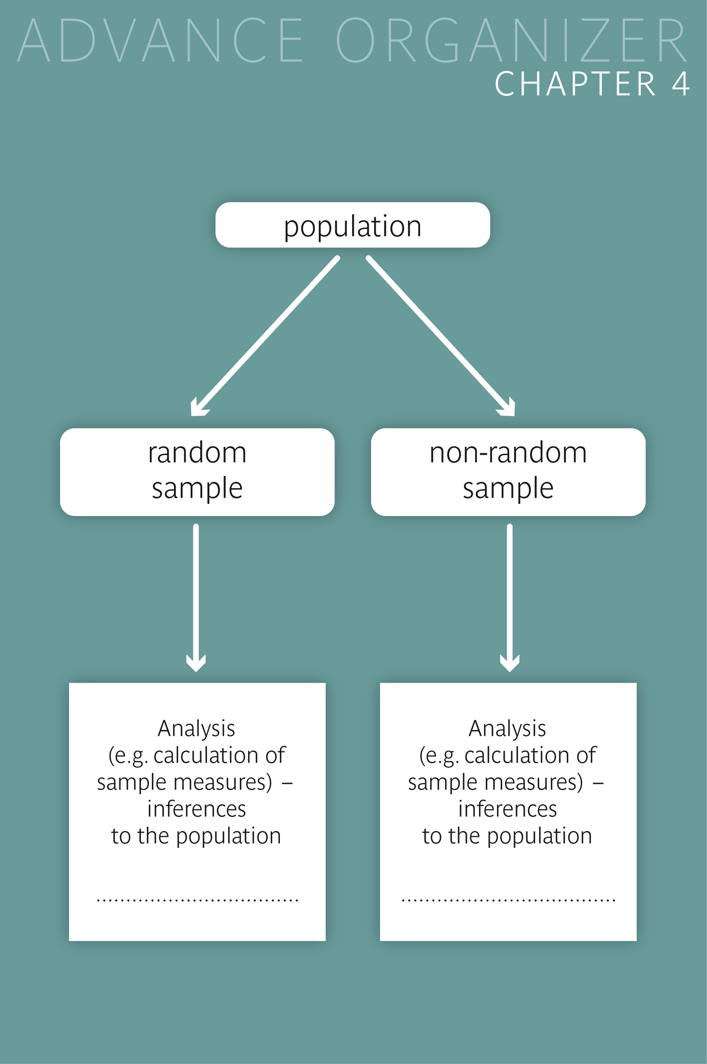
Question 4.2.1 addresses the problem of generalizing results obtained in specific samples to a broader population. In the following we will formulate the problems encountered in this example in a more general way.
Let us start with the following general question: When are we allowed to make statements about population parameters on the basis of sample statistics? In a concrete example this might read: When can the mean value \( \bar{x} \) and the standard deviation \( s_{X} \) of a quantitative variable \(X\) in a given sample be used to draw conclusions on the respective parameters \( \mu_{X} \) and \( \sigma_{X} \) of the population from which the sample was drawn?
In order to clearly distinguish sample statistics and population parameters, Greek letters are used for population parameters, e.g. \( \mu \) to denote the mean value and \( \sigma \) to denote the standard deviation of a variable at the population level. If it is unclear from the context, which variable \(X\) is meant, it is advisable to provide the symbols \( \mu \) and \( \sigma \) with a respective subscript, as we did in the beginning. These population parameters are fixed and do not depend on chance.
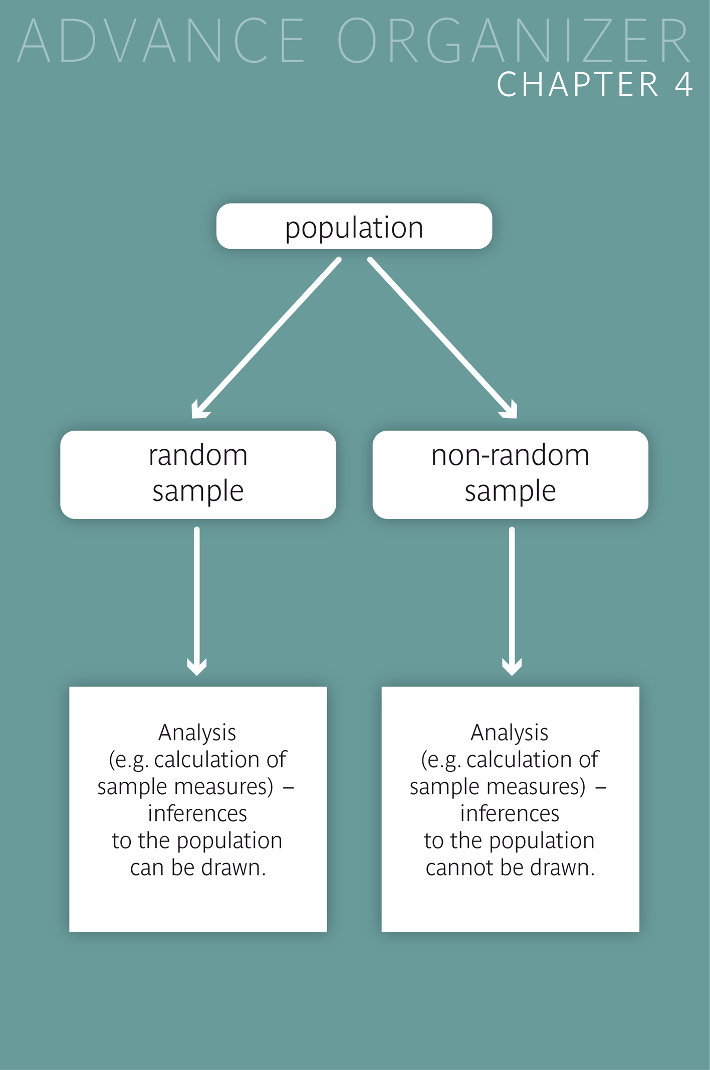
It is clear that the results of a sample cannot be generalized to any population. In general, the sample should at least be a subset of the population of interest. However, this is not sufficient. The elements of the sample should be selected randomly. This is the case with Dr. Frank N. Stein's sample which represents a random selection of employees of the chemical company. Hence Dr. Stein is allowed to draw conclusions from his sample to the population of all employees of the company and to estimate parameters of this population based on the respective statistics of his sample.
|
Synopsis 4.2.1
If a sample represents a random selection of a population of interest, the population parameters may be estimated based on the resspective sample statistics. |
Question 4.2.1 shows that such estimations can be problematic if the sample does not represent a random selection from the population of interest. The percentage of women is clearly smaller in Dr. Stein's sample than in the total population. Therefore the mean weight is higher in his sample than in the total population. Based on this sample, we would thus overestimate the mean body weight of the total population.
We speak of a "biased" estimate, if a population parameter is systematically over- or under-estimated. Such a systematic estimation error is called "bias". If we presume that women have an average weight of \(62 kg\) and men an average weight of \(76 kg\) and that there is an equal number of women and men in the total population, the mean value of weight of the adult population would be \(69 kg\). The mean value of \(74 kg\) from Dr. Stein's sample would exceed this population value by \(5 kg\) and the bias would be \(5 kg\) in this case.
Estimates generally deviate from the the respective population parameters to some extent. However, as long as these deviations are due to chance alone, the estimates are unbiased. The concept of bias is sharpened in the following definition.
|
Definition 4.2.1
Let \( \Theta' \) denote the value which would be obtained on average, if an estimation procedure for the population parameter \( \Theta \) of interest were repeated over and over again. The difference \( \Theta' - \Theta \) is the bias of the estimation procedure. |
|
Definition 4.2.2
An estimation method is called "unbiased" if its bias equals \(0\). An estimation method is called "consistent", if the bias gets smaller and smaller with increasing sample size. |
The classical method to estimate populatin parameters is to draw a random sample from the respective population and to calculate the respective sample statistics. This provides estimates with the smallest possible bias. For mean values and variances, even small random samples provide unbiased estimates, and this is also true for relative frequencies. However, standard deviations provide consistent but not unbiased estimates.
|
Definition 4.2.3
A sample is said to be representative of a population, if its statistics differ little from the respective population parameters. |
Therefore, a sample providing biased estimates of the respective population parameters is not representative of the underlying population, unless these biases are small. In general, the representativity of a sample can only be guaranteed if its elements are drawn randomly. However, this is not sufficient. In order to provide precise estimaties, a sample also needs to have a sufficient size. We will see this in chapter 8.

The major goal of survey design is to ensure that (sufficiently) precise estimates of important population parameters will be obtained. The following two subchapters address this topic.
Ideally, we deal with a population which is homogeneous. In this case we can assume that the measures of interest do not systematically vary between sub-groups of the population, and we can draw a simple random sample. As we have already seen, it is important that the sample is drawn randomly, because factors associated with the selection process (e.g., age, gender, education) might otherwise lead to biased results.
The following example illustrates that systematical estimation errors can indeed be avoided by randomly drawing the sample.
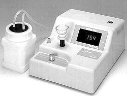
called "Cyanmethemoglobin spectrophometer"
While he mean level of haemoglobin of Dr. Stein's \(121\) patients equals \(159.5 mg/dl\), the mean level of the population of all \(3488\) chemical company employees equals \(158.7 mg/dl\). Apparently Dr. Stein's estimate, based on his \(121\) clients, is quite accurate in this case.
However, this cannot be taken for granted, if we consider that there are systematic differences in the haemoglobin level of women and men. In fact, the sub-group of \(590\) women in the population of chemical company employees has a mean haemoglobin level of \(143.9 mg/dl\), while the mean haemoglobin level of the \(2898\) men is \(161.7 mg/dl\). Thus, the population is inhomogeneous regarding the variable "haemoglobin".
The reason why Dr. Stein's estimate of the mean haemoglobin level is nevertheless quite accurate is that the allocation of the employees to the medical practitioners happened randomly. Therefore, the distribution of gender in his sample corresponds quite well to the one in the population.
Dr. Stein wants to estimate the mean body height of all employees of the chemical company without measuring each and everyone of them individually. Here, we have to be aware of the important effect of the gender ratio on the mean body height. Hence Dr. Stein chooses his sample in such a way that the ratio between men and women, which is approx. \(5 : 1\) in the population, is also reflected in his sample. He decides to randomly select \(90\) men (i.e., five times the number of women in his sample) and then caculates the mean body height of these \(90\) men and of the \(18\) women.
As with a simple random sample, he will again obtain an unbiased estimate of the mean value of the population. However, since the gender distribution of the sample coincides with the one at the population level and cannot be different by chance, the estimate of the mean height in this stratified random sample is likely to come closer to the mean value of the population than the mean value of height in the simple random sample of \(121\) employees.
Alternatively, Dr. Stein might have calsculated a so-called "weighted mean" \[ \frac{5}{6} \times \bar{x}_{1} + \frac{1}{6} \times \bar{x}_{2} \] of the mean value \(\bar{x}_{1}\) of height in the \(103\) men and the mean value \(\bar{x}_{2}\) of height in the \(18\) women. By using the proportions of men (\(\frac{5}{6}\)) and women (\(\frac{1}{6}\)) in the underlying population as weights of the observed gender-specific means, an unbiased estimate of mean height at the population level is obtained.
In this way, Dr. Stein would have been able to use the data of all \(103\) men of his sample.
|
Synopsis 4.2.2
If the elements of the population differ in factors, which are (or might be) related to the variable of interest, the respective population is inhomogeneous. In this case it is advisable to draw a stratified random sample. To do so, the population is divided (stratified) into sub-populations which are as homogeneous as possible. From each of these sub-populations we then draw a random sample whose size is proportional to the size of the respective sub-population. Sometimes a sub-population is over-sampled on purpose. In this case, the sub-samples must not be pooled. Instead, the statistic of interest (e.g., a mean or a proportion) must first be calculated for each of the sub-samples separately. In a second step, a weighted mean of the sub-sample statistics is computed, with the weights assigned to the sub-sample statistics being proportional to the sizes of the corresponding sub-populations. |
|
Synopsis 4.2.3
The accuracy of estimates can be improved with a careful survey design. |
With the following applet you can draw simple and stratified random samples.
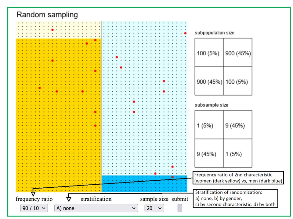
Samples can be drawn from a population of \(2000\) subjects (represented by tiny dots), of which \(1000\) are women (yellow part) and \(1000\) are men (blue part). A second characteristic (dark colors) has a total relative frequency of \(50\%\). The frequencies of this second characteristic may be chosen to differ between men and women (left drop down list). You may draw
Moreover, you may choose between different sample sizes (3rd drop down list). By testing different combinations of the three input parameters (distribution of the second characteristic in men and women, type of randomisation and sample size) try to answer the question: "When is stratified random sampling clearly superior to simple random sampling".
Here, we leave out an important element of survey design, i.e., the determination of sample size. We will consider this aspect in more detail in chapter 9. For now, a simple principle must do:
A larger sample size generally improves the accuracy of estimates provided that these are unbiased.
Unplanned studies are an ideal breeding ground for biased results. Often, these are studies, for which the data already exist and the drawing of a random sample is no longer possible. Caution is needed when interpreting statistical results from such studies, as these are often not generalisable.
On the other hand, studies in which samples are drawn randomly according to a predefined survey design are much less susceptible to biases.
Since biased sample results can rarely be corrected in retrospect, the time invested in a good survey design is well worth the effort.
"Experimental studies" are a special category of planned studies. The characteristic of an experimental study is that specific (experimental) factors influencing the outcome of interest can be allocated to the experimental units by the experimenter (we speak of experimental rather than of observational units in this case).
If the experimental units are different (as is the case in studies with humans or animals), experimental factors are usually randomly allocated (randomised) to the experimental units. In this way, the distribution of the factors can be controlled by the experimenter.
Here, we use the term "factor" for a variable that can influence a specific outcome of interest. For instance, in a drug trial, the values of the factor "drug" are the different drugs tested. To be precise, we should say that the values of a factor are allocated to the experimental units (e.g., the different drugs studied). However, "factor allocation" is used for simplicity.
On the other hand, studies, in which the values of the factors of interest are "natural" properties of the observational units, are referred to as "observational studies". In such studies, the distribution of the factors of interest is predetermined by "nature" and cannot be changed (e.g. we cannot determine whether a person ought to smoke or not). In this case, we speak of "personal factors". Two examples will illustrate the difference between personal and experimental factors:
(i) The influence of age on blood pressure shall be studied. Clearly, age is a personal factor, as it can not be changed. This study is therefore observational.
(ii) In order to test the effectiveness of a new drug, \(50\) persons are randomly selected from a population of \(100\) patients and are then treated with the drug, while the remaining patients are given a placebo. The type of treatment drug/placebo can be arbitrarily (ideally randomly) allocated to the study subjects and is thus an experimental factor. This study is therefore experimental.
The study design underlying the second example will now be treated in more detail.
If the two groups differ in a relevant outcome after having been treated with the drug resp. the placebo during a certain period of time, then these differences can only be explained by the different experimental conditions of the two groups and/or by chance.
If we knew that the differences are not explained by chance alone, could we then infer that the drug and placebo have different effects? The answer is "not necessarily".
In clinical studies, subjective perception (on the side of the patient and of the attending physician) can creep in as biasing factor. We have to consider that patients who know that they were given a placebo may feel worse than those getting the drug.
In order to eliminate such biases, clinical studies are carried out in a "double-blind" fashion, whenever possible. Neither patients nor physicians are then allowed to know who is taking the drug and who the placebo. This means that the randomisation key (i.e., the key for the group allocation, generated using a chance mechanism) must be kept secret and that the preparations of the experimental drug (also referred to as "verum") and of the placebo must not be distinguishable from outside.
and the placebo
must not be distinguishable
from the outside.
Patients who are randomised in the context of a clinical trial usually do not represent a random sample of a larger patient population. Often, they are recruited in one or more hospitals during a certain time period. The randomisation of this collective into two equally sized groups can be achieved by drawing a random sample of half the size of the collective, whereby the patients of the random sample form one group and the other patients the other group.
If more than two groups should be formed, several random samples must be drawn. For instance, if we want to randomise \(100\) patients into \(4\) groups of equal size, we first have to draw a random sample of \(25\) people from the \(100\) patients, then another random sample of \(25\) people from the remaining \(75\) patients, and finally a third random sample of \(25\) people from the \(50\) patients remaining after the second draw.
|
Definition 4.3.1
The random partition of a study population into two or more subgroups of a predefined size is called "simple randomisation". |
As in the case of random samples, it can be advantageous to carry out a stratified randomisation. Here, randomisation is done separately in different sub-groups of patients. These sub-groups might be
In this way, the different experimental groups will look the same or almost the same regarding the stratification variables. With simple randomisation, however, such variables may end up having slightly different distributions in the different experimental groups, which may bias the results of the experiment. For instance, if younger patients respond better to the experimental drug than older ones and the proportion of younger patients is higher / lower in the group receiving the experimental drug, the effect of the drug will be over- / under-estimated.
Remark: That the collective of patients to be randomised is known in advance, is the ideal situation. In general, however, patients are recruited consecutively. In this case, patients are divided into consecutive blocks of a given size \(B\) (e.g., \(B = 4\)), and randomisation is done by block. Thus, if two equally sized groups are to be formed and \(B = 4\), each of the two groups must have \(2\) patients in each of the blocks.
Only randomly drawn samples guarantee that the sample statistics obtained provide valid estimates of the respective population parameters. Here, "valid" means that the value of the sample statistic differs only randomly but not systematically from the respective population parameter. Such estimates are called "unbiased". Mean values, variances and relative frequencies can be estimated without bias even from small random samples.
In the case of a biased estimate, the bias is defined as the difference between the mean value of the estimate across all possible equivalent random samples and the true value of the population parameter.
In heterogeneous populations, the variability of the sample estimates can be reduced by drawing separate random samples from homogeneous sub-populations.
Chance (or random) is also used as a methodical element in experimental studies, in which the experimental units (mostly patients or healthy subjects in medical research) are randomly allocated to the different treatments. As in the case of stratified random samples, results can be improved by stratified randomisation (i.e., by conducting randomisation separately in different sub-groups of patients).