Chapter 6

The normal distribution

We need models in order to structure the almost infinite number of possibie distributions of continuous variables. Even though these models always provide simplified descriptions of reality, they enable general statements which could not be made otherwise. In this chapter, the normal distribution is introduced as a model for many continuous quantitative variables, e.g., body height, haemoglobin level, etc..

6.1. The concept of a model distribution

The distribution of a variable is the frequency pattern of its values in the population. This frequency pattern can be graphically illustrated, based on data from a random sample, a) with a bar chart for qualitative variables and b) with a histogram for quantitative variables. However, as no two random samples are the same, such descriptions are only suitable to a limited extent for generalisations and predictions. To overcome this difficulty, mathematical models are used in statistics. Although they are simplified representations of reality, they can often provide valid predictions. In some ways, models can be compared to clothes which are produced in a limited number of shapes and sizes but still fit a multitude of slightly different body shapes.

6.2 The central role of the normal distribution

The normal distribution (or - to use a more popular term - the Gaussian bell curve) is of central importance in statistics due to various reasons:

a) The frequency distribution of many quantitative variables (e.g. body height, haemoglobin level, etc.) can be described in good approximation with a Gaussian bell curve.

b) The random deviations of many sample statistics (mean values, proportions, percentiles, etc.) from the respective unknown population parameters can often be described in good approximation by a Gaussian bell curve, provided that the samples are of sufficient size.

Example:

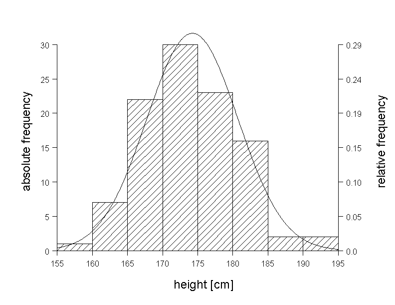
In figure 6.2 we can see a histogram of the body height of the 103 male chemical company employees, with a Gaussian bell curve superimposed to it. This curve represents an idealisation of the histogram, as it smoothes its random irregularities. The area under the bell curve equals the total area of the histogram. Hence, the shaeded bar sections above the curve sum up to the same area as the white area sections underneath the curve.

In principle, individual values \( x \) of a continuous variable \( X \) appear with a probability of \(0\) (points do not have any extension). Therefore the y-coordinates \( f(x) \) of the Gaussian bell curve cannot be interpreted as probabilities or frequencies. In fact, \( f(x) \) indicates the density of the values of the random variable \( X \) at \(x\). In statistics, such curves are called "probability density functions" or just "density functions". Positive probabilities only result when considering intervals instead of points. The probability of \( X \) having a value in the interval \([a, b]\) is given by the area under the curve \( f(x) \) between \( a \) and \( b \). Let this area be denoted by \(I(a,b)\). Then the ratio \(\frac{I(a,b)}{b-a}\) is the average probability density of \(X\) in the interval \([a, b]\). If we now let the interval \([a, b]\) shrink to the point \(a\), then the ratio \(\frac{I(a,b)}{b - a}\) converges to \(f(a)\). Thus, \(f(a)\) is the probability density of \(X\) at \(a\).

If we consider the Gaussian bell curve as an approximation to the histogram, we can expect the relative frequency of the observed values lying within the interval \( [a, b] \) to be approximately equal to \(I(a,b)\). Let the area of the histrogram between two limitis \(a\) and \(b\) be denoted by \(H(a,b)\). If we choose, for example, \( a = 167.5 \) cm and \( b = 172.5 \) cm, then \(H(a,b) = 0.25\) (black area in the left graph of figure 6.3). The corresponding area \(I(a,b)\) under the Gaussian bell curve (black area in the right graph of figure 6.3) is \(0.24\). The areas \(H(a,b)\) and \(I(a,b)\) also agree well for other intervals \([a,b]\).

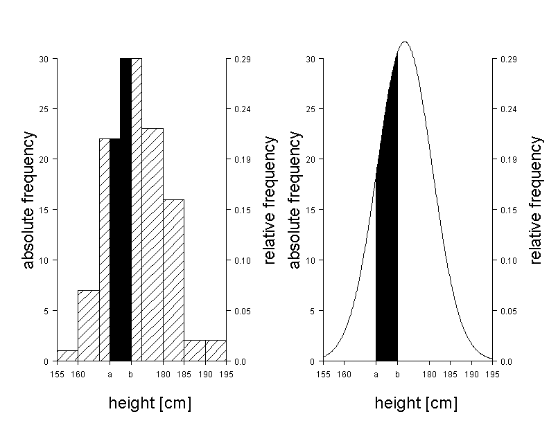
This supports the assumption that the Gaussian bell curve is suitable for the description of the distribution of body height in the population.

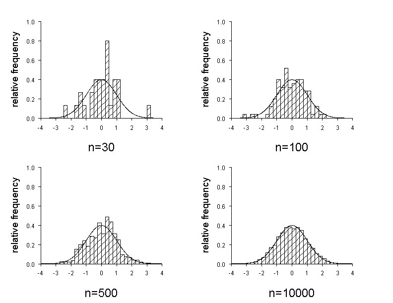
Figure 6.4 shows how the histogram of a normally distributed variable \( X \) approaches the Gaussian bell curve with increasing sample size. To illustrate this, normally distributed random samples of the sizes \( n = 30, 50, 100 \) and \( 10000 \) were generated and a histogram was drawn for each sample size, with the corresponding Gaussian bell curves superimposed to it. We notice that the deviations between the bell curve and the histogram are very small for \( n = 10000 \).

6.3. A short profile of the normal distribution

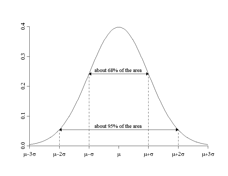
The density function of the normal distribution is symmetrical and bell- shaped and is also called "Gaussian bell curve". In figure 6.5, the Gaussian bell curve1 is illustrated.

The Gaussian bell curve is given by the equation \[ f(x) = \frac{1}{\sqrt{2\pi}\times\sigma} \times e^{\Large{\frac{1}{2}\times(\frac{x-\mu}{\sigma})^2}} \]

6.4 The central role of the standard normal distribution

In primciple, the parameters \( \mu \) and \( \sigma \geq 0\) can be varied arbitrarily. Hence, there is an infinity of specific normal distribution models. However, the model with \( \mu = 0 \) and \( \sigma = 1 \) is of central importance.

We will see that all other normal distribution models can be linked to this standard model. But to begin with, work through rhe following two questions concerning the standard normal distribution. They can be answered using the applet "Standard Normal Distribution".

6.5 An elegant method to estimate quantiles

Dr. Frank N. Stein wants to know if his son, who is \(1.86 m\) tall, lies above the 90th percentile of the body height of adult men. He assumes that the body height of men is approximately normally distributed with a mean of \(176\) cm and a standard deviation of \(7\) cm. In an appendix of statistical tables of one of his books, he finds a value of \( z_p = 1.28 \) for the \(90\)-th percentile (or the \(0.9\)-quantile) of the standard normal distribution. (The \(p\)-quantile of the standard normal distribution is usually denoted by \( z_p \)). You can get this value using the applet "Standard normal Distribution.

Dr. Stein knows that the standard deviation of the standard normal distribution is \(1\) and concludes that the \(90\)-th percentile must thus lie \(1.28\) standard deviations above the mean. As a result he gets: \[ P90 = 176 + 1.28 \times 7 = 185 \] . His son's body height lies thus above the 90th percentile.

6.6 Reference (or normal) ranges in Medicine and other empirical sciences

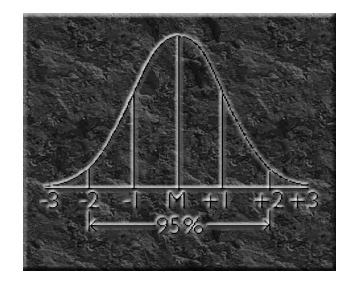
Reference ranges (or normal ranges) of medical variables are often defined by determining specific percentiles as "limits of normal". If a large enough random sample is available, it may be possible to estimate the respective percentiles directly from this random sample, without any model assumptions, by following the rules from chapter 3. However high and low sample percentiles (e.g., \(P95\) and \(P5\)) often show considerable deviations from the respective true values in the population, even for relatively large random samples. The method for estimating percentiles inroduced just before often provides more reliable results, provided that the normal distribution is a good model for the data. This also explains why normal ranges are often defined using the formula \( \mu \pm 2\sigma \) in Medicine. For a normally distributed variable approx. \(95 \%\) of all observations lie in this range. Such normal or reference ranges are said to be two-sided.

Often, however, only deviations from the mean value in one direction matter. For example Dr. Stein was notified by his colleague, the respiratory physician Dr. B. Ventura, that one of his patients, Mr. X, lies below the lower limit of normal of forced vital lung capacity for men of his age and height. The sex-, age- and height-dependent lower limits of normal are defined by the respective \(5\)-th percentiles or the \(0.05\)-quantiles in a population of non-smokers without breathing problems. We know from the Swiss SAPALDIA-study (Swiss Study on Air Pollution and Lung and Heart Diseases in Adults) that the forced vital lung capacity of male non-smokers without breathing problems is approximately normally distributed with a mean value dependent on age and height and a constant standard deviation of \(0.62\) litres.

Here, a concluding remark is in order: it does not always make sense to define normal ranges based on percentiles. It matters more whether values of the respective variable above or below a certain level are associated with an increased health risk. However, such questions are often hard to answer, since a clear line between high and low to moderate risks can seldom be drawn.

6.7 Reduction of infinitely many models to one single model

In the following sections, we will see how the distribution of an arbitrary normally distributed variable can be linked to the standard normal distribution.

6.7.1. Standardisation transformation:

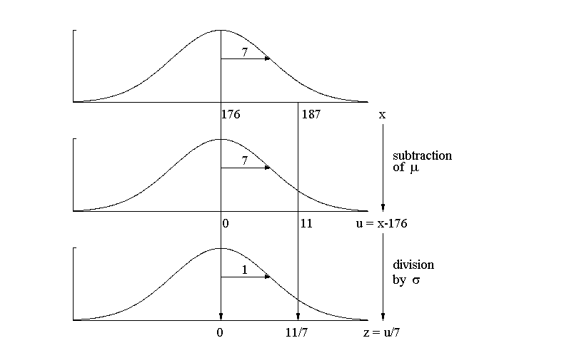
The following figure is based on the normal distribution model of body height with \( \mu = 176\) cm and \( \sigma = 7\) cm. It shows how a normally distributed variable \( X \) can be transformed to a standard normally distributed variable \( Z \). We assume a concrete value of \( x = 187\) cm and then get the respective quantile z of the standard normal distribution in two steps.

The most obvious advantage of this transformation is that it enables reducing all probability calculations for normally distributed variables to the standard normal distribution. Hence a single table is sufficient for all such calculations. You can find such a table in any statistics text book. Alternatively, you can use the Excel-function \(NORM.DIST(z;0;1;1)\) to calculate probabilities \(P(Z \leq z)\) and the Excel-function \(NORM.INV(p;0;1)\) to determine \(p\)-quantiles for a variable \(Z\) with a standard normal distribution. Of course, you can also use the applet "Standard normal distribution". However, the values provided by this applet do not have the same level of accuracy for values of \(z\) with \(|z| > 3.7\) or \(P(Z < z) < 0.0001\) as the values provided by the two Excel-functions.

Exercise :

We want to estimate the percentage of men with a body height between \(175\) cm and \(185\) cm. Try to reproduce the following steps by using the applet "Normal Distribution". Again, we assume that the mean and the standard deviation of body height in men are \(176\) cm and \(7\) cm, respectively, and we denote male body height by \( X \).

1. Calculation of the probability that \( X \leq 185 \), denoted by \( P(X \leq 185) \):

First we transform \( x = 185 \) to \( z = (185 - 176)/7 = 1.286 \).

Then we have \( P(X \leq 185) = P(Z \leq 1.286) \) = area underneath the standard bell curve up to \( z = 1.28 = 0.901 \) (as we can find using the applet "Standard normal distribution".

2. Calculation of the probability that \( X \leq 175 \) denoted by \( P(X \leq 175) \):

The transformation of \( x = 175 \) results in \( z = (175 - 176)/7 = -0.143 \).

Hence we have \( P(X \leq 175) = P(Z \leq -0.143) = \) area underneath the standard bell curve up to \( z = -0.143 = 0.443 \).

3. Calculation of the probability that \( 175 \leq X \leq 185 \):

This probability is the difference between the probabilities of 1) and 2), which equals \( 0.90 - 0.443 = 0.458 \) .

According to this estimate, slightly less than \(50 \%\) of men would be between \(175\) cm and \(185\) cm tall.

To be precise, the above probability is \( P(175 \lt X \leq 185) \) and not \( P(175 \leq X \leq 185) \). However, the two probabilites are the same because the probability \( P(X = 175) \) equals \(0\) if we assume \( X \) to be continuous.

6.8 How can the normal distribution assumption be verified?

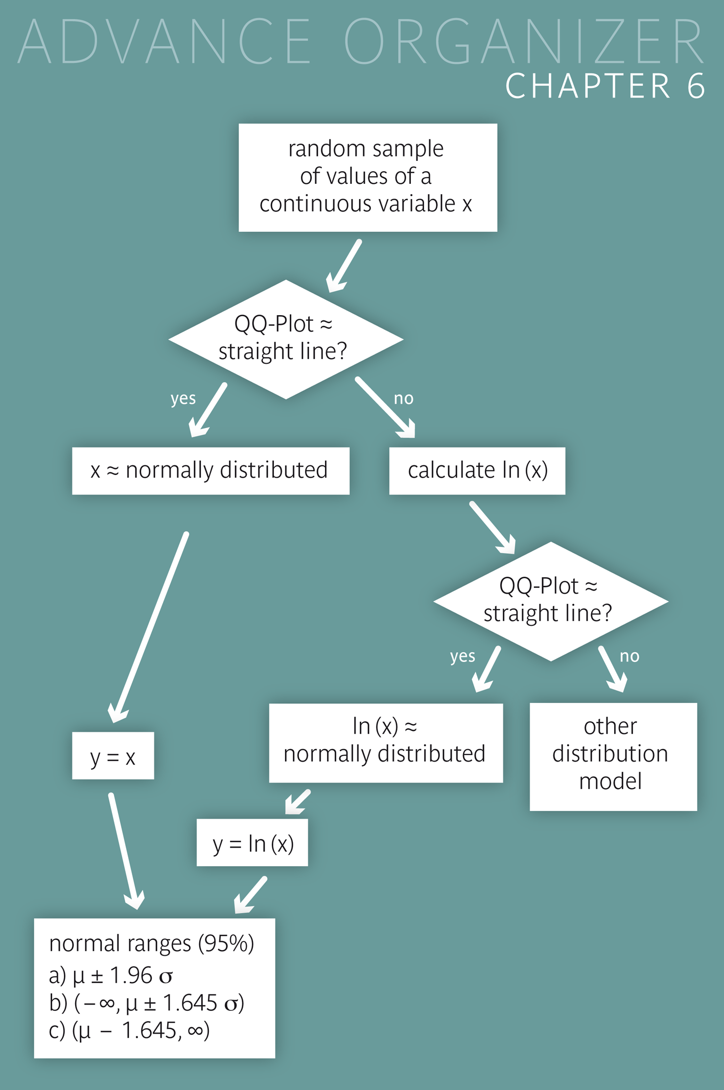
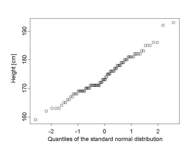
Up to now we have just assumed that the variables considered were approximately normally distributed. Of course this assumption has to be verified. This can be done visually with the so-called "quantile-quantile plot" (short: Q-Q plot). In the Q-Q plot, the sample quantiles \( x_p \) (cf. chapter 3) are plotted against the theoretical quantiles \( z_p \) of the standard normal distribution. More precisely, the \(k\)-th value of the ascendingly ordered sample \( x_{[k]} \) is matched to the quantile \( z_{(k-0.5)/n} \) of the standard normal distribution. For instance, if \(n = 50\), the \(20\)-th observation of the ordered sample (which approximately corresponds to the \(40\)-th percentile) is matched to the quantile \( z_{0.39} \) and the \(45\)-th observation of the ordered sample (which approximately corresponds to the \(90\)-th percentile) is matched to the quantile \( z_{0.89} \). If the resulting points form approximately a straight line, up to some random fluctuations, the respective variable can be considered as normally distributed. This is the case with body height of the male chemical company employees.

The Q-Q plot of the body mass index of the 18 female chemical company employees attended to by Dr. Stein shows a different picture:

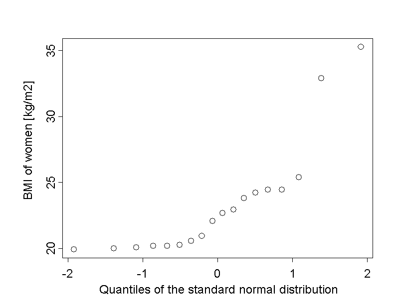
Here, the points form a curved line. This points to an asymmetrical distribution. The upward curvature indicates that the dispersion of the data increases with growing values of body mass index (right-skewed distribution).

6.9 The logarithmic transformation

For many variables \( X \) with a right-skewed distribution, a logarithmic transformation (short: log-transformation) can lead to an approximately symmetrical, or even an approximately normal distribution of the data. If the logarithmised variable \( Y = ln(X) \) approximately follows a normal distribution, its two-sided \(95 \%\)-reference range can be estimated using the standard procedure. By transforming back the limits of the reference range of \( Y \), we obtain limits of the \(95 \%\)-reference range of \( X \).

For math enthusiasts : In principle, the choice of the natural logarithm \( y = ln(x) \) is optional. We could also choose the common decadian logarithm. The back transformation would then be carried out with the function \( 10^{()} \). However, the choice of \( y = ln(x) \) offers interpretational advantages, which can be seen when dealing more deeply with these issues.

Example

The logarithmised values of the leukocyte counts of the chemical company employees attended to by Dr. Stein have a mean of \(4.176\) and a standard deviation of \(0.304\). We can assume that the distribution of log-transformed counts is approximately normal. Therefore, the \(95 \%\)-reference range for leukocyte counts can be estimated at \[ (e^{4.176 - 1.96 \times 0.304} , \, e^{4.176 + 1.96 \times 0.304}) = (35.9, \, 118.1) \] In reality, \(4.1 \%\) of the vlues are higher than \(111.6\) and \(1.7 \%\) of the values are lower than \(35.3\) in this sample. Hence \(94.2 \%\) of all 121 values lie between the limits of \(35.9\) and \(118.1\). The empirically defined limits of this reference range (defined by the \(2.5\)-th and the \(97.5\)-th empirical percentile) are \(38\) and \(122\), respectively. Some differences can thus be observed between the two alternative results.

On the other hand, the value \( e^{4.176} = 65.1 \), which can be used to estimate the median of the number of leukocytes, corresponds quite well to the sample median of \(63\). In fact, for this method to provide an unbiased estimate of the median of \( X \), it is sufficient that the values of the log-transformed variable \( Y = ln(X) \) have a symmetrical distribution.

6.10. Summary

The normal distribution (whose probability density function is often referred to as Gaussian bell curve) provides a model for the description of many quantitative variables. Each normal distribution model is uniquely defined by the mean value \(\mu\) and the standard deviation \(\sigma\). If a variable \(X\) has an approximate normal distribution, then approx. \(2/3\) of its values fall into the interval \([\mu - \sigma, \, \mu + \sigma]\) and approx. \(95 \%\) into the interval \([\mu - 2 \times \sigma, \, \mu + 2 \times \sigma]\).

Any normal distribution with parameters \( \mu \) and \( \sigma \) can be linked to the standard normal distribution with a mean of \( \mu = 0 \) and a standard deviation of \( \sigma = 1 \) via the z-transformation \( Z = \frac{X-\mu}{\sigma} \). This transformation (also referred to as "standardisation") is used to compute probabilities for normally distributed variables.

The inverse transformation \( X = \mu + Z \times \sigma \) is used to compute percentiles of normally distributed variables. If \(z_p\) is the \(p\)-quantile of the standard normal distribution, then \( \mu + z_p \times \sigma \) is the \(p\)-quantile or \((100 \times p)\)-th percentile of \(X\). The most important quantiles of the standard normal distribution are tabulated in any text book of statistics.

With the help of the standard normal distribution, reference (or normal) ranges can be defined for variables whose distribution is approximately normal.

The Q-Q plot enables a visual assessment of the normal distribution assumption for a random variable \( X \). Assuming a normal distribution is plausible, If the dots of the Q-Q plot lie approximately on a straight line. This assessment is however inevitably subjective, so that the use of formal statistical tests of normality can sometimes be indicated.