
|
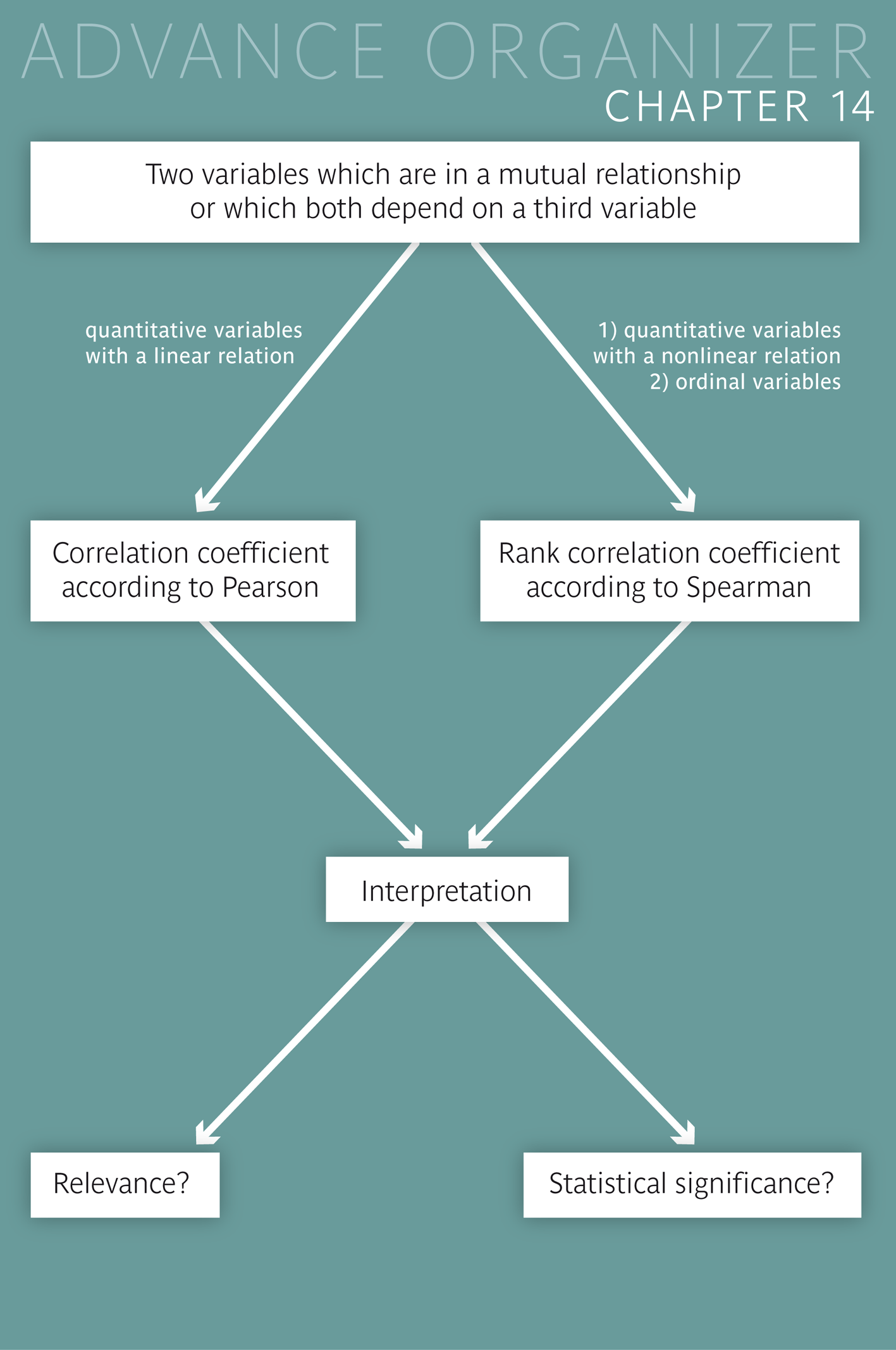
Often, there is no one-directional relation between two quantitative variables \(Y\) and \(X\). For instance, this is the case, if the two variables mutually influence each other or if they both depend on a third variable \(Z\) or several common determinants. In such cases, the correlation is either described by the classical correlation coefficient of Pearson or by Spearman's rank correlation coefficient. |
|
Educational objectives
You are familiar with Pearson's correlation coefficient and you can explain what it expresses. You can explain the idea of the coefficient of determination of a simple linear regression model and can calculate it from the correlation coefficient. You are familiar with the most important properties of Pearson's correlation coefficient. You can explain what it means if the correlation coefficient has a value of \(1\) or \(-1\) and you know different situations in which the correlation coefficient is \(0\). You are also familiar with situations in which a high correlation coefficient does not reflect a linear relation between the two variables. You know how and under which conditions the hypothesis of a linear correlation between two quantiative variables can be tested. You are furthermore familiar with Spearman's rank correlation coefficient, which can measure linear and non-linear relations between numerically and ordinally scaled variables. You can explain what the extreme values \(1\) or \(-1\) mean with the rank correlation coefficient. You can decide in which cases the rank correlation coefficient should be preferred to the classical correlation coefficient. Key words: linear relation, variance explained, coefficient of determination, Pearson's correlation coefficient, Spearman's rank correlation coefficient Previous knowledge: scatter plot (chap. 2), mean value, standard deviation, variance (chap. 3), normal distribution, Q-Q plot (chap. 6), hypotheses, \(p\)-value (chap. 9), regression line, slope parameter (chap. 13) Central questions: How can the correlation between two quantitative variables be measured if neither of them takes the role of the dependent or independent variable? |
In keeping with the methods of the preceding chapter, the mean value of the diastolic blood pressure (\((Y\) ) might be described as a linear function of the systolic blood pressure (\(X\)). But the roles of the two variables could also be interchanged and the mean value of \(X\) could be modeled as a linear function of \(Y\) . Theoretically speaking, the roles of blood volume \(Y\) and body weight \(X\) could have also been interchanged in the preceding chapter. However this would have made little sense since body weight is a more fundamental variable than blood volume, and it is easy to determine.
The following plots show the two blood pressure values of Dr. Frank N. Stein's \(121\) chemical company employees. The left scatter plot describes the dependency of the diastolic blood pressure on the systolic blood pressure and the right scatter plot the dependency of the systolic blood pressure on the diastolic blood pressure. The two superimposed regression lines are denoted by \(g_{Y|X}\) and \(g_{X|Y}\) in the following.
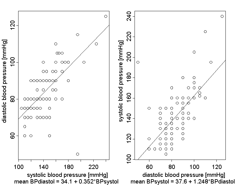
In general, the two regression lines \(g_{Y|X}\) and \(g_{X|Y}\) have different slopes \(\hat{\beta}_{Y|X}\) and \(\hat{\beta}_{X|Y}\). Therefore, a natural idea is to calculate the geometric mean of the two slopes as a measure for the linear relation between \(X\) and \(Y\). This mean is defined as follows: \[\sqrt{\hat{\beta}_{Y|X} \times \hat{\beta}_{X|Y}}\] (The geometric mean of two positive numbers \(a\) and \(b\) is defined as the positive square root of their product: \(GM(a, b) = \sqrt{a\times b}\)).
In our example we get \(\sqrt{0.352 \times 1.248} = 0.663\) as geometric mean of the two slopes \(\hat{\beta}_{Y|X} = 0.352\) and \( \hat{\beta}_{X|Y} = 1.248 \).
But what if the two slopes are not positive?
If both slopes are negative (i.e., if both lines are decreasing), then the geomtric mean of the absolute values of their slopes is calculated and the root is endowed with a negative sign. In fact the two slopes always have the same algebraic sign, it is not possible that one slope is positive and the other one negative.
The geometric mean of the ahsolute values of the two slopes endowed with the algebraic sign of the slopes coincides with the so-called "Pearson correlation coefficient", whose computation formula is given in the mathematical appendix of the chapter.
This correlation measure, which is commonly denoted by \(r\), was first proposed by the French physicist Auguste Bravais in 1844 and then later re-discovered by Karl Pearson.
Pearson's correlation coefficient is a measure of the strength of the linear relation between \(X\) and \(Y\). Its value always lies between \(-1\) and \(+1\) and takes the extreme values \(1\) and \(-1\), if and only if the points of the scatter plot define an increasing or decreasing straight line, respectively.
The following figure shows different scatter plots representing linear relations of varying strength between the two variables \(X\) and \(Y\).
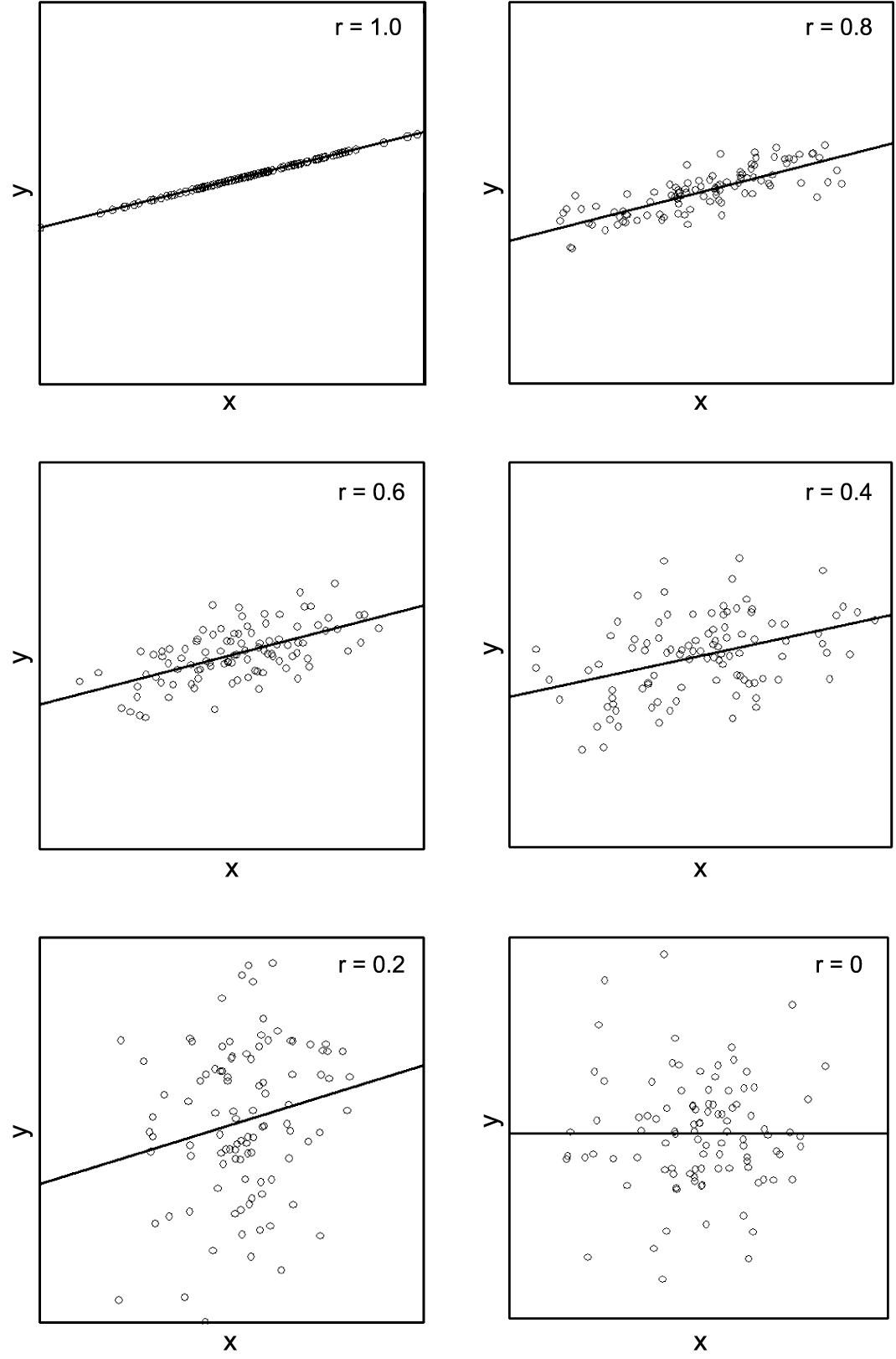
The illustrated correlations range between \(r = 1\) in the upper left plot and \(r = 0\) in the lower right plot. With the exception of the last scatter plot, all others have regression lines with a positive slope. Furthermore we notice that, in all diagrams, the points are about equally distributed in \(y\)-direction on both sides of the regression line.
Except for the case in which \(r = 0\), we are looking at situations in which there is a more or less strong positive linear relation between the variables \(X\) and \(Y\). In the extreme case with \(r = 1\), the points lie exactly on a straight line (perfect linear relation). In the other extreme case, the regression line runs horizontally and we cannot see any relation between \(X\) and \(Y\) . In the first case, the complete information about \(Y\) is already contained in \(X\). (If we know the value of \(X\), we can immediately calculate the value of \(Y\).) In the example with \(r = 0\), however, \(X\) does not contain any information about \(Y\).
These statements also apply if the roles of \(X\) and \(Y\) are interchanged.
Under certain conditions, the correlation coefficient is thus a measure of how much information the two variables \(X\) and \(Y\) contain about each other. If \(r = 1\) and the two variables define a straight line, then each one of them contains the complete information (\(100\%\)) about the other one. In the other extreme case, the two variables contain no information (\(0\%\)) at all about each other. The restriction "under certain conditions" is justified. We will soon encounter an example in which \(Y\) is completely determined by \(X\) and yet \(r = 0\) holds. But before, we take a look at analogue scatter plots with negative linear relations between \(X\) and \(Y\) of different strength.
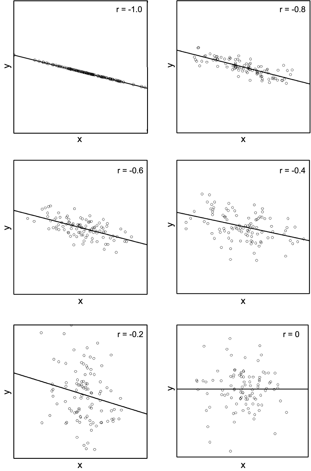
In this case, the correlation coefficients have a negative algebraic sign because of the negative relation between \(X\) and \(Y\).
As regards the information shared by \(X\) and \(Y\) the same statements as before apply. The following figure illustrates these issues
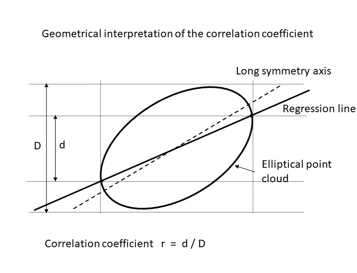
The scatter plot is schematically illustrated as an ellipse. In reality, many scatter plots have approximately this shape. In particular, this is the case if the two variables \(X\) and \(Y\) originate from a two-dimensional normal distribution and if the sample size is not too small.
We notice that the regression line differs from the long symmetry axis of the ellipse. The regression line cuts the boundary of the ellipse at the points with the most extreme \(x\)-coordinates. On the inside of the ellipse, the \(y\)-values of the regression line vary within an interval of length \(d\). The \(y\)-coordinates of the points of the ellipse however spread across a larger interval of length \(D\). In fact, the ratio between \(d\) and \(D\) equals the correlation coefficient \(r\).
If the scatter plot has a negative slope, then \(r\) is negative. In this case, \(r = - \frac{d}{D}\). We can thus say that the absolute value of the correlation coefficient indicates the proportion of the dispersion of \(Y\) that is described by the regression line between \(Y\) and \(X\).
In a scatter plot with a regression line \(y = \hat{\alpha}_{Y|X} + \hat{\beta}_{Y|X} \times x\), we can, for each data point \((x_i, y_i)\), determine the corresponding point \( (x_i,\hat{\alpha}_{Y|X} + \hat{\beta}_{Y|X} \times x_i) \) on the regression line (i.e., the point with the same \(x\)-coordinate). The \(y\)-coordinate \(\hat{\alpha}_{Y|X} + \hat{\beta}_{Y|X} \times x_i\) of this point is usually denoted by \(\hat{y}_i\). In the following schematic figure a scatter plot with three points and the corresponding regression line is shown. The observed values \(y_i\), the respective predicted values \(\hat{y}_i\), as well as the residuals \(e_i = y_i - \hat{y}_i\) are labeled.
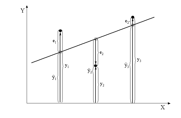
If only \(x_i\) were known, then \(\hat{y}_i\) would be predicted for \(y_i\). Therefore \(\hat{y}_i\) is also called the part of \(y_i\) explained by \(x_i\). Accordingly the residual \(e_i = y_i - \hat{y}_i\) is the part of \(y_i\) which is not explained by \(x_i\).
We are now interested in the comparison between the standard deviation of the values \(y_i\) and the standard deviation of the values \(\hat{y}_i\) (standard deviation of the values \(\hat{y}_i\). This leads us to the following synopsis:
|
Synopsis 14.2.1
The following statements apply to the absolute value of the correlation coefficient \(r\): \[ |r| = \frac{\text{standard deviation of the values} \,\, \hat{y}_i}{\text{standard deviation of the values} \,\, y_i} \] The absolute value of the correlation coefficient \(r\) thus indicates the proportion of the standard deviation of \(Y\) which is explained by \(X\) via the regression line \(g_{Y|X}\). The same applies if the roles of \(X\) and \(Y\) are interchanged, i.e. \(|r|\) also indicates the proportion of the standard deviation of \(X\) which is explained by \(Y\) via the regression line \(g_{X|Y}\). |
For the sake of simplicity we often omit "via the regression line", as in the formula above. But this is only appropriate if the scatter plot between \(Y\) and \(X\) does not show any curvature.
What is the concrete meaning of the above synopsis for our example?
Based on the result of \(r = 0.663\), systolic blood pressure explains a proportion of \(0.663\) or \(66.3\%\) of the standard deviation of diastolic blood pressure. Conversely, the same percentage of the standard deviation of systolic blood pressure is explained by diastolic blood pressure.
Since the variance is equal to the square of the standard deviation, the preceding synopsis can be reformulated as follows:
|
Synopsis 14.2.2
The square \(r^2\) of the correlation coefficient of \(X\) and \(Y\) indicates the proportion of the variance of \(Y\) which is explained by \(X\) via the regression line \(g_{Y|X}\). Conversely, \(r^2\) also indicates the proportion of the variance of \(X\), which is explained by \(Y\) via the regression line \(g_{X|Y}\). |
The square \(r^2\) of the correlation coefficient is also called the "coefficient of determination" or "R-squared" of the regression model \(g_{Y|X}\) (or \(g_{X|Y}\)) (in this context, "determined" has the meaning of "explained").
We can thus also say that systolic blood pressure of our example explains a proportion of \(0.6632^2 = 0.439\) or \(43.9\%\) of the variance of diastolic blood pressure. Conversely, the same percentage of the variance of systolic blood pressure is explained by diastolic blood pressure.
In the jargon of statistics: the coefficients of determination of the two linear regression models describing the dependency of one blood pressure variable on the other one have the same value \(0.439\).
Another important interpretation of the correlation coefficient is given in the following synopsis:
|
Synopsis 14.2.3
The correlation coefficient of \(X\) and \(Y\) indicates by how many standard deviations \(s_Y\) of \(Y\) the value of \(Y\) predicted by \(g_{Y|X}\) changes, if the value of \(X\) is increased by one standard deviation \(s_X\). Since the correlation coefficient does not depend on the order of the variables, \(X\) and \(Y\) can switch roles in this statement as well. |
In our example, this means that value of diastolic blood pressure prediced by systolic blood pressure increases by \(0.663\) standard deviations (i.e by \(0.663 \times 12.3 = 8.2\) mmHg), if the value of systolic blood pressure is increased by one standard deviation (i.e., by \(23.2\) mmHg).
First of all we summarise which statements can be made without examining a scatter plot in the extreme cases of \(r = 1, r = -1\) and \(r = 0\).
|
Synopsis 14.3.1
The following statements apply to Pearson's correlation coefficient:
|
In all other cases, the respective scatter plot should be examined in order to interpret the correlation coefficient. The four scatter plots in the following figure illustrate that we need to pay attention when interpreting a correlation coefficient
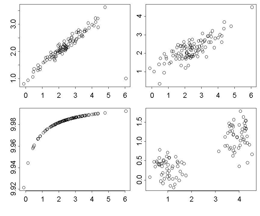
The correlation coefficient \(r\) equals \(0.8\) in all four cases. The relation is quite linear in the two upper scatter plots. In the upper left scatter plot the points scatter more tightly around a straight line than in the upper right plot. What lowers the correlation coefficient to 0.8 is one single outlying point in the lower right corner of the plot.
In the lower left scatter plot, there is an exact functional relation between \(Y\) and \(X\): the points lie on a segment of a parabola. In this case the value of one variable can always be determined from the value of the other variable. Each variable thus carries the complete information about the other one. Here, the correlation coefficient is smaller than \(1\) because the points do not lie on a straight line.
In the lower right scatter plot we can see two completely separated scatter plots, inside which no relation between \(X\) and \(Y\) exists. We should thus keep in mind the following rule:
|
Synopsis 14.3.2
A high correlation coefficient between two variables \(X\) and \(Y\) does not imply that there is an almost linear relation between \(X\) and \(Y\). |
Now we turn to the example where \(r = 0\) holds, despite the fact that \(X\) contains the complete information about \(Y\).
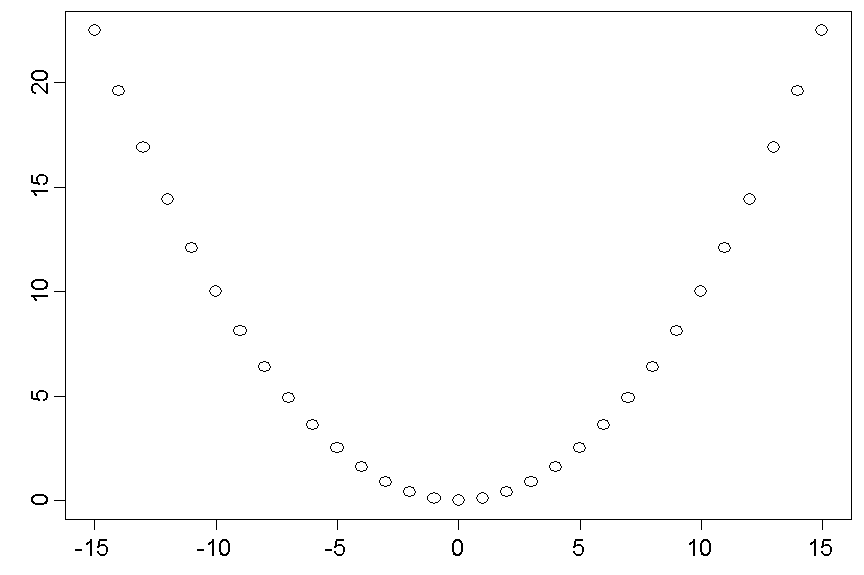
The points lie symmetrically on a parabola \(y = 0.1 \times x^2\).
The symmetry of the set of points with respect to the vertical line at \(x = 0\) implies that the regression line \(g_{Y|X}\) has a slope of \(0\). The slope of \(g_{X|Y}\) equals \(0\) as well. This follows from the fact that \( x = \pm \sqrt{y}\), implying that the prediction of \(x\) given \(y\) must be \([\sqrt{y} + (-\sqrt{y}]/2 = 0\). Hence \(g_{X,Y}\) is the horizontal line at the level \(0\).
As both slopes equal \(0\), their geometric mean must be \(0\) as well, implying that the correlation coefficient of \(X\) and \(Y\) equals \(0\). Nevertheless \(y\) is completely determined by \(x\). For example, the \(y\)-value belonging to \(x = 10\) must be \(0.1 \times 10^2 = 10\). We can thus also state:
|
Synopsis 14.3.3
A correlation coefficient of \(0\) does not imply that there is no relation between the two variables \(X\) and \(Y\), it only implies that there is no linear relation between them. |
These examples show that one should always examine the underlying scatter plot when interpreting a correlation coefficient
With the applet "Pearson correlation" you can explore the properties of the Pearson correlation coefficient \( r \) and of the coefficient of determination \(r^2\).
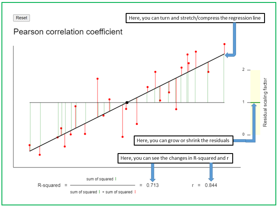
In the applet "Pearson correlation coefficient", you can explore the properties of the Pearson correlation coefficient. By seizing one of the ends of the black regression line, you can rotate the line or stretch or crush it in horizontal or vertical direction. When doing this, the residuals remain unchanged, i.e., the points keep their original vertical distance from the regression line. With the black ruler on the right hand side, one can grow or shrink the residuals. The effects of these interventions on the Pearson correlation coefficient r and its square, R-squared, can be observed at the bottom. To illustrate the definition of R-squared, the residuals are represented as red arrows ranging from the regression line to the respective point, and the predicted values on the regression line as green arrows ranging from the mean level to the regression line.
Try to observe what happens with R-squared and the Pearson correlation coefficient r
a) when you rotate the regression line.
b) when you stretch or crunch the regression line in vertical direction.
c) when you stretch or crunch the regression line in horizontal direction.
d) when you grow or shrink the residuals.
The correlation coefficient is a pure number, a so-called dimensionless measure. In our example of blood pressure, we would thus always get the same value, irrespective of the pressure scale used (e.g., mmHg, mbar or P).
Even if we describe the relation between body height and body weight, the correlation coefficient does not depend on the choice of the units used for the height and weight measurements.
Changes in the zero point of the measuring scale do not affect the correlation coefficient either. For instance, if we compared two methods of measuring fever by performing both measurements in each patient, then the correlation coefficient of the two measurements would not depend on the temperature scale chosen. We could even express the meassurements of one method in \(^{\circ} C\) and the ones of the other method in \(^{\circ} F\) (Fahrenheit).
However the correlation coefficient does change if we change from a linear to a non-linear scale. If we compared the two inflammation markers CRP (C-reactive protein) and ESR (erythrocyte sedimentation rate) of patients, we would no longer get the same correlation coefficient if we took the logarithmised values of CRP and ESR instead of the original values.
|
Synopsis 14.4.1
The correlation coefficient is a dimensionless measure. It does not depend on the scales used to measure \(X\) and \(Y\), as long as corresponding scales are linked by a linear equation, i.e., as long as \[ \text{value on scale 2} = a + b \times \text{value on scale 1} \,\,\, \text{(with} \, b \gt 0) \,. \] |
In the example of the temperature scales \(^{\circ} C\) (scale 1) and \(^{\circ} F\) (scale 2), the linear equation is given by \(a = 32\) and \(b = 1.8\).
In chapter 13, the \(p\)-value of the slope \(\hat{\beta}\) of a regression line was introduced. Likewise we can speak of the \(p\)-value of a correlation coefficient \(r\). The null hypothesis, under which the \(p\)-value is calculated, states that, in reality, there is no relation between the variables \(X\) and \(Y\). The \(p\)-value equals the probability that a correlation between \(X\) and \(Y\) at least as strong as the one observed had to be expected under the null hypothesis (i.e., as a result of chance alone).
The definition of \(|r|\) as geometric mean of the absolute values of the two slopes \(\hat{\beta}_{Y|X}\) and \(\hat{\beta}_{X|Y}\) suggests a direct connection between the significance of the correlation coefficient and the significance of the two slopes. In fact, the \(p\)-value of the correlation coefficient is identical to the \(p\)-value of the two slopes. However, strictly speaking, this \(p\)-value is only valid, if the two variables \(X\) and \(Y\) are close to normally distributed and their scatter plot has approximately the shape of an ellipse.
To simplify matters we assume that these conditions are fulfilled in our example.
In our concrete problem, the null hypothesis is:
There is no relation between the systolic and the diastolic blood pressure in the population of the Basel chemical company employees (i.e., none of the two variables carries any information on the other one).
while our alternative hypothesis is:
There is a linear relation between systolic and diastolic blood pressure, with a correlation coefficient \(\rho \neq 0\), in the population of the Basel chemical company employees.
Notice that the negation of the null hypothesis would be that there is a relation between the two variables. This would also include situations, in which the relation is non-linear. However, as we are only interested in linear relations for now, it is more precise to speak of "our hypothesis".
Now let's take a look at the results of the regression model between diastolic blood pressure and systolic blood pressure, as they might be displayed by a statistics program:
| variable | parameter estimate | standard error | t-value | p-value |
| intercept | 34.11 | 5.276 | 6.4651 | \(\lt 0.001\) |
| BDsystol | 0.3516 | 0.0365 | 9.6442 | \(\lt 0.001\) |
The estimated slope of the regression line between diastolic and systolic blood pressure equals \(0.352\) and its \(p\)-value is \(\lt 0.001\).
|
Synopsis 14.5.1
The null hypothesis that there is no relation between two quantitative variables \(X\) and \(Y\) at the population level (i.e., that none of them carries any information about the other one), can be tested as follows in a random sample: We test if the slope of the regression line between \(Y\) and \(X\) (or between \(X\) and \(Y\) ) differs significantly from \(0\) or not at the given significance level. This test provides valid conclusions, if the variables \(X\) and \(Y\) are both close to normally distributed and the scatter plot has approximately the shape of an ellipse. Since a non-linear relation between \(Y\) and \(X\) is not compatible with these conditions, the test should only be applied if no relation at all or an approximately linear relation can be recognised between the two variables in the scatter plot. |
Beware:
The assessment of a correlation coefficient should not only be based on the \(p\)-value. In large samples, even very small correlation coefficients may differ significantly from \(0\). In such a situation the relevance of the respective correlation should be questioned (cp. chapter 9).
In chapter 11, you were introduced to the procedure of ranking sample values (in connection with the Wilcoxon rank-sum test). This approach can also be applied to describe relations between two variables. To do so, we substitute the \(x\)- and \(y\)-values by their respective ranks:
The smallest \(x\)-value gets rank \(1\), the second smallest rank \(2\), etc., and the same procedure is applied to the \(y\)-values. If a value occurs more than once, the respective ranks are averaged. In this case, one speaks of "ties".
If we do not use the original values of \(X\) and \(Y\) for the calculation of the correlation coefficient, but their ranks, we get "Spearman's rank correlation coefficient", which is often denoted by \(r_S\).
|
Synopsis 14.6.1
If the relation between two variables \(Y\) and \(X\) is not linear or if the variables are not normally distributed, then Spearman's rank correlation coefficient provides an alternative correlation measure. In principle, it is calculated like the classical correlation coefficient, with the difference that the original observations of \(X\) and \(Y\) are replaced by their ranks in the ordered samples. Therefore, the rank correlation coefficient is less sensitive to outliers than the classical correlation coefficient. |
In our example, the value of the rank correlation coefficient is \(0.678\) and thus very similar to the one of the classical correlation coefficient (\(0.663\)).
With a \(p\)-value \(\lt 0.0001\), the rank correlation coefficient of the two blood pressure measures also differs highly significantly from \(0\). Since the \(p\)-value of the rank correlation coefficient is valid under very general conditions, we can no longer doubt, even from a purely statistical point of view, that there is indeed a relation between the two blood pressure variables.
We will now look at the values which the rank correlation coefficient \(r_S\) takes in the four examples with a Pearson correlation coefficient of \(0.8\).
Spearman's correlation coefficients for the four examples are the following:
In the upper left figure, the rank correlation coefficient \(r_S\) is larger than the classical correlation coefficient \(r\), since \(r_S\) is hardly influenced by the outlier in the lower right corner.
The figure on the lower left shows that the rank correlation coefficient can also be equal to \(1\) if the points do not lie on a straight line.
Furthermore the rank correlation coefficient is clearly smaller than the classical correlation coefficient in the example with the two separate point clusters.
In order to correctly understand the difference between Pearson's and Spearman's correlation coefficient, we have to find out when the rank correlation coefficient equals \(1\).
According to its definition, this is the case, if the ranks of the \(x\)- and \(y\)-values define an increasing straight line. One can prove mathematically that this line must then be the identity line. Thus, the ranks of the \(x\)- and the \(y\)-values must be the same in all observational units.
In order for the ranks of the \(x\)- and the \(y\)-values to exactly agree, the original points \((x_i,, y_i)\) must lie on an increasing polygonal line without horizontal and vertical segments. This explains why the rank correlation coefficient is equal to \(1\) in the lower left plot. Hence the rank correlation coefficient cannot only identify linear relations, but it equals \(1\) whenever the \(x\)- and the \(y\)-values define the exact same order among the observational units.
If Pearson's correlation coefficient and Spearman's rank correlation coefficient have similar values, this indicates that the relation between the two variables is close to linear. In the the example of systolic and diastolic blood pressure this is indeed the case.
The fact that the rank correlation coefficient cannot be equal to \(1\) or \(-1\) if the polygonal line defined by the points contains horizontal or vertical segments, is due to the fact that
|
Synopsis 14.6.2
The following statements hold for Spearman's rank correlation coefficient:
|
To conclude this section we want to ask ourselves what the \(p\)-value of a rank correlation coefficient means.
To find out, we assume that the \(x\)- and the \(y\)-values are detached from their "owners" and then randomly permuted between the different persons of the sample. As a consequence, a true relation would no longer exist between the two measurements and the rank correlation coefficient could only randomly differ from \(0\).
The \(p\)-value of a given observed rank correlation coefficient equals the probability that a random permutation of the underlying \(x\)- and \(y\)-values would produce a rank correlation coefficient at least as different from \(0\) as the one initially observed. A low \(p\)-value thus provides evidence for the hypothesis that there is a real relation between the two observed variables.
Since ranks represent ordinal data, the rank correlation coefficient can also be applied to describe relations between ordinal variables (at least if the number of levels of the variables is reasonably large).
Example:
Two doctors have to judge the severity of a disease in \(20\) patients independently of one another, on a scale with \(6\) levels (\(0\) = disease absent, \(1\) = light form of the disease, ..., \(5\) = most severe form of the disease)
| Patient | Doctor 1 | Doctor 2 | Rank 1 | Rank 2 |
|---|---|---|---|---|
| 1 | 1 | 2 | 1.5 | 4.5 |
| 2 | 3 | 3 | 9 | 9 |
| 3 | 4 | 5 | 13.5 | 18 |
| 4 | 5 | 5 | 18.5 | 18 |
| 5 | 3 | 4 | 9 | 13.5 |
| 6 | 4 | 2 | 13.5 | 4.5 |
| 7 | 5 | 5 | 18.5 | 18 |
| 8 | 2 | 1 | 5 | 1.5 |
| 9 | 2 | 2 | 5 | 4.5 |
| 10 | 5 | 4 | 18.5 | 13.5 |
| 11 | 1 | 1 | 1.5 | 1.5 |
| 12 | 2 | 3 | 5 | 9 |
| 13 | 4 | 3 | 13.5 | 9 |
| 14 | 4 | 4 | 13.5 | 13.5 |
| 15 | 2 | 2 | 5 | 4.5 |
| 16 | 5 | 5 | 18.5 | 18 |
| 17 | 3 | 3 | 9 | 9 |
| 18 | 2 | 3 | 5 | 9 |
| 19 | 4 | 5 | 13.5 | 18 |
| 20 | 4 | 4 | 13.5 | 13.5 |
In this example the rank correlation coefficient is \(0.81\) and its \(p\)-value is \(\lt 0.001\).
|
Synopsis 14.7.1
Unlike Pearson's correlation coefficient, Spearman's rank correlation coefficient can also be applied if the two variables \(X\) and \(Y\) are ordinal or if one of the variables is quantitative and the other one is ordinal. |
When calculating the regression line and the correlation coefficient, the so-called covariance plays an important role. We assume that we measured two variables \(X\) and \(Y\) in \(n\) individuals (e.g. the systolic and the diastolic blood pressure). With \(x_1, x_2, ..., x_n\) we denote the measured values of the variable \(X\) and with \(y_1, y_2, ..., y_n\) the measured values of the variable \(Y\), the subscripts indicating the persons to which the respective values belong. The sample means of \(X\) and \(Y\) are denoted as usual by \(\bar{x}\) and \(\bar{x}\). The sample variances of \(X\) and \(Y\) are calculated as follows (as we have seen in chapter 3): \[ s_X^2 = \frac{(x_1-\bar{x})(x_1-\bar{x})+(x_2-\bar{x})(x_2-\bar{x})+...+(x_n-\bar{x})(x_n-\bar{x})}{n-1} \] \[ s_Y^2 = \frac{(y_1-\bar{y})(y_1-\bar{y})+(y_2-\bar{y})(y_2-\bar{y})+...+(y_n-\bar{y})(y_n-\bar{y})}{n-1} \] The covariance may be thought of as being the child of the two variances. With each observational unit it inherits one factor from \(s_X^2\) and one factor from \(s_Y^2\). \[ s_{XY} = \frac{(x_1-\bar{x})(y_1-\bar{y})+(x_2-\bar{x})(y_2-\bar{y})+...+(x_n-\bar{x})(y_n-\bar{y})}{n-1} . \] Since the order of the factors does not affect the value of the product, \(s_{YX}\) has the same value as \(s_{XY}\) . In the sequel we will thus only use \(s_{XY}\). The correlation coefficient is now mathematically defined as \[ r = \frac{s_{XY}}{s_X \times s_Y} \] where \(s_X\) and \(s_Y\) denote the sample standard deviations of \(X\) and \(Y\), respectively. Furthermore the following equations hold: \[ \hat{\beta}_{Y|X} = \frac{s_{XY}}{s_x^2} \] and, by symmetry, \[ \hat{\beta}_{X|Y} = \frac{s_{YX}}{s_Y^2} = \frac{s_{XY}}{s_Y^2} \] We can now see why \(|r|\) is equal to the square root of the product of the two slopes \[ \begin{aligned} \sqrt{\hat{\beta}_{Y|X} \times \hat{\beta}_{X|Y}} & = \sqrt{\frac{s_{XY}}{s_X^2} \times \frac{s_{XY}}{s_Y^2}} \\ & = \frac{s_{XV}}{s_X \times s_Y} \end{aligned} \] We now imagine a situation in which a partial loss of data has left us with the values of \(X\). If we have previously calculated \(s_X\), \(s_Y\) and \(s_{XY}\), we can then at least try to estimate the \(y\)-values as follows: \[\hat{y_i}= \hat{\alpha}_{Y|X} + \hat{\beta}_{Y|X} \times x_i \] Since \(\hat{\alpha}_{Y|X} \) is a fixed number, the standard deviation of the values \(\hat{y_i}\) equals \(\hat{\beta}_{Y|X} \times s_X\). The ratio between this standard deviation and the standard deviation of the original \(y\)-values is equal to \[ \frac{s_{\hat{y}}}{s_y} = \hat{\beta}_{Y|X} \times \frac{s_X}{s_Y}\] If we now substitute \(\frac{s_{XY}}{s_X^2} \) for \(\hat{\beta}_{Y|X}\), we get \[ \frac{s_{\hat{y}}}{s_y} = \hat{\beta}_{Y|X} \times \frac{s_X}{s_Y} = \frac{s_{XY}}{s_X^2} \times \frac{s_X}{s_Y} = \frac{s_{XY}}{s_X \times s_Y} = r \] By symmetry, the same statements hold if the roles of \(X\) and \(Y\) are interchanged. Therefore the statements of synopsis 14.2.1 are proved. The formulas listed above also show how the slope of the regression line can be calculated from the correlation coefficient and the standard deviations of \(X\) and \(Y\). In fact, the following additional formula holds: \[ \hat{\beta}_{Y|X} = r \times \frac{s_Y}{s_X} \]
If there is a linear relation between two quantitative variables \(X\) and \(Y\), then its strength is measured by Pearson's correlation coefficient. The values of the correlation coefficient can vary between \(-1\) and \(1\). If the correlation coefficient equals \(1\) or \(-1\), then there is an exact linear relation between the values of \(X\) and \(Y\). In this case, the points of the scatter plot of \(Y\) and \(X\) define a straight line which increases if \(r = 1\) and decreases if \(r = -1\).
If there is no relation between \(X\) and \(Y\) at the population level, then their correlation coefficient in a random sample can only differ from \(0\) by chance. Whether or not an observed correlation coefficient between \(X\) and \(Y\) differs significantly from \(0\), can be assessed by testing if the slope of the regression line between \(Y\) and \(X\) differs significantly from \(0\). For this test to be valid, however, the two variables should be close to normally distributed and their scatter plot should have approximately the shape of an ellipse.
The square of the correlation coefficient \(r\) (also referred to as "R-squared" or "coefficient of determination") indicates the proportion of the variance of \(Y\) which is explained by the regression line between \(Y\) and \(X\). Conversely, the proportion of the variance of \(Y\) which is unexplained by the regression line equals \(1-r^2\). It equals the ratio between the variance of the residuals and the variance of \(Y\). By symmetry, these statements also hold if the roles of \(X\) and \(Y\) are interchanged.
Apart from Pearson's classical correlation coefficient, Spearman's rank correlation coefficient also plays an important role. It can be used in a more general context and should be applied if
Furthermore, the rank correlation coefficient can be tested against \(0\) without having to impose any validity conditions on the distributions of \(X\) and \(Y\).
As a rule, a correlation coefficient different from \(1\) or \(-1\) should never be interpreted without looking at the underlying scatter plot.