Chapter 7

The binomial distribution

If we are interested in the probability for a specific outcome to occur \(x\) times in a series of \(n\) independent and identical random experiments, the answer is provided by the binomial distribution. This could be the total number of occurrences of the number \(6\) in \(n\) throws of a die or the total number of people with a specific characteristic in a random sample of size \(n\).

7.1. The binomial distribution

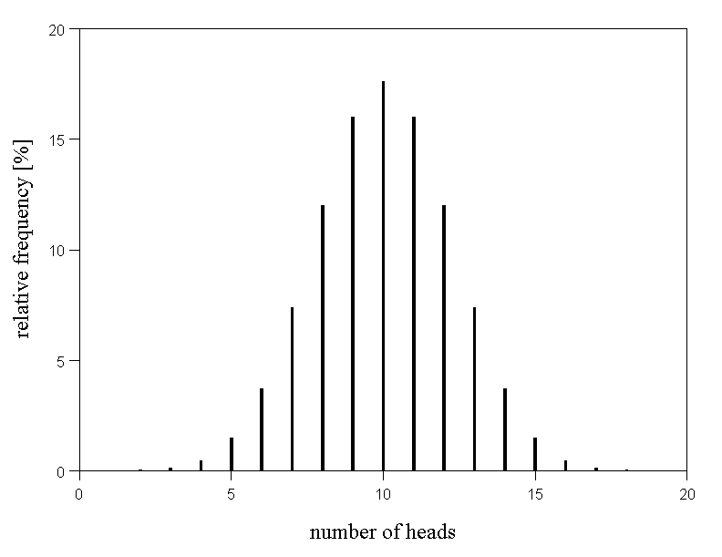
If a fair coin is tossed \(n\) times and \(n\) is sufficiently large, we will generally observe about the same number of "heads" and "tails". We thus expect to get about \( n/2 \) times head and \( n/2 \) times tail. Although the count (number) \( X \) of heads can vary in a relatively wide range, large deviations from the value \( n/2 \) are rare.

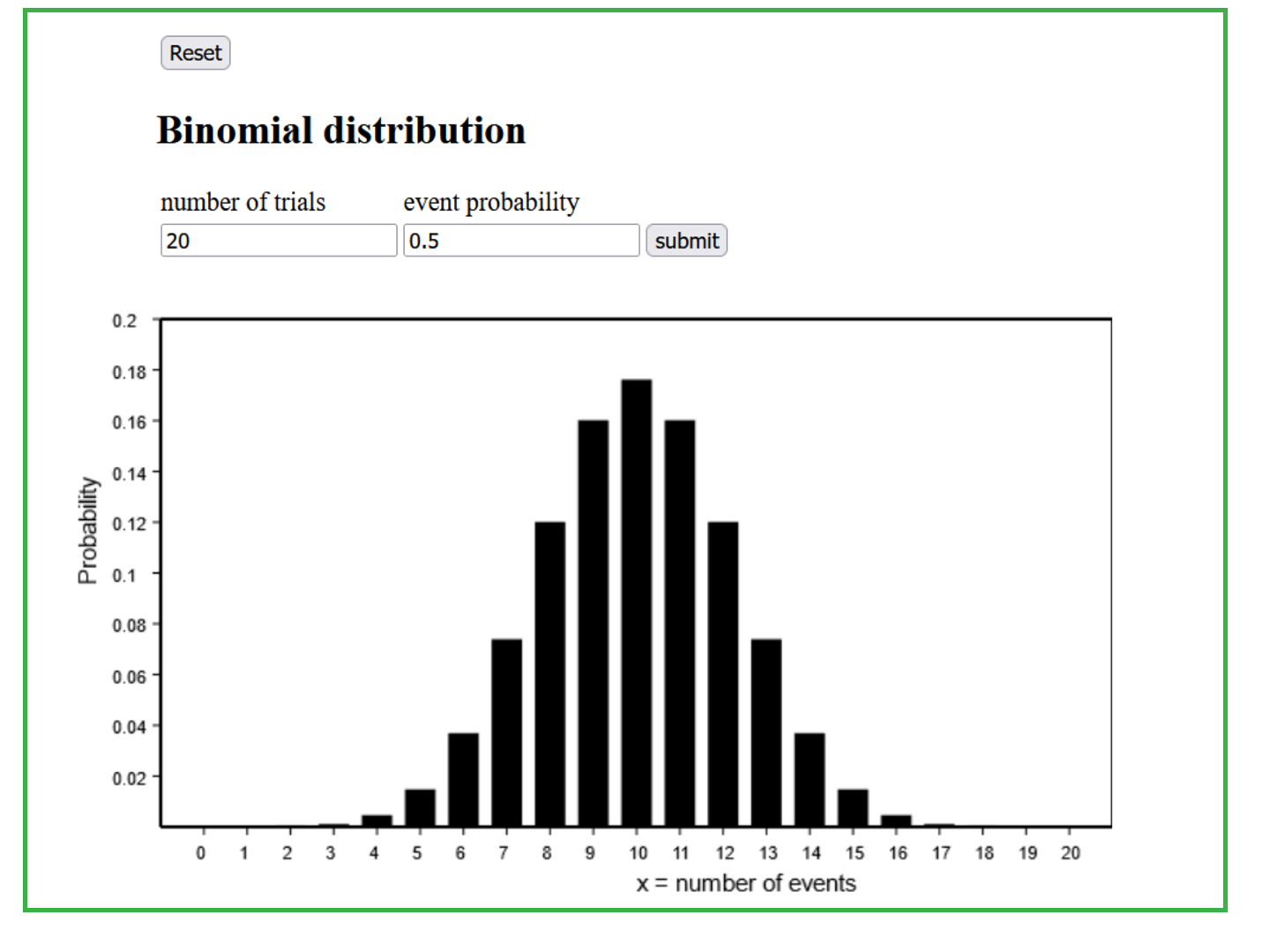
The frequency distribution of the count of heads among \( n = 20 \) tosses in a very large (i.e., ideally infinite) number of repetitions of \( n = 20 \) tosses is illustrated in the following diagram. It shows the probabilities of the so-called "binomial distribution" with the parameters \( n = 20 \) (number of repetitions of the random experiment - in our case the tossing of a coin) and \( \pi = 0.5 \) (probability of the outcome of interest in each random experiment). This probability distribution is symmetrical and the value occurring most often is \(10\).

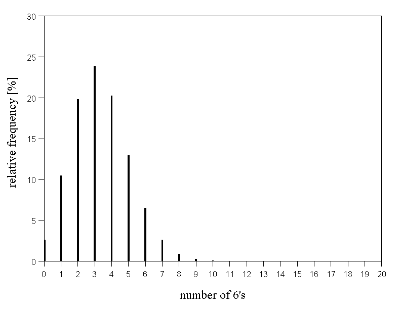
Another classical random experiment is the repeated throwing of a die, where we may count the number of sixes. The probability to get a six in one throw is \( 1/6 \). How often do we e.g. get exactly seven sixes, only sixes or no sixes at all in a series of 20 throws of the die? We thus ask for the probability distribution of the number of sixes in a series of \(20\) throws of a die.

Figure 7.3 below illustrates the probability distribution of the number of sixes in a series of \(20\) throws. We notice that the probability of only getting sixes is very small. (The bar at \(20\) is too small to be visible.) The same is already true for values bigger than nine. The most frequent values are \(3\) and \(4\). They are the integer neighbours of \( 20/6 = 3.333... \). Accordingly, the probability distribution is asymmetrical.

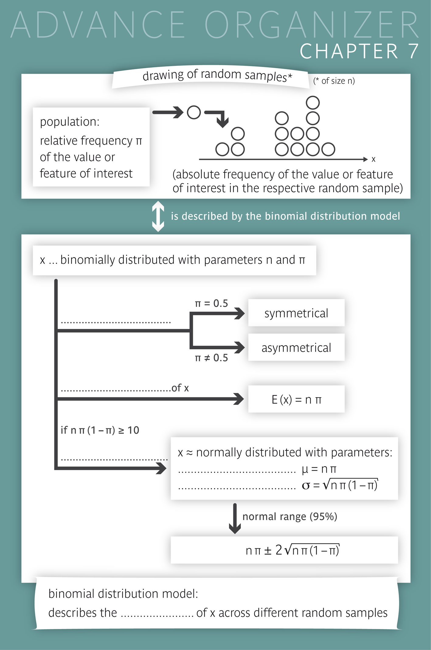
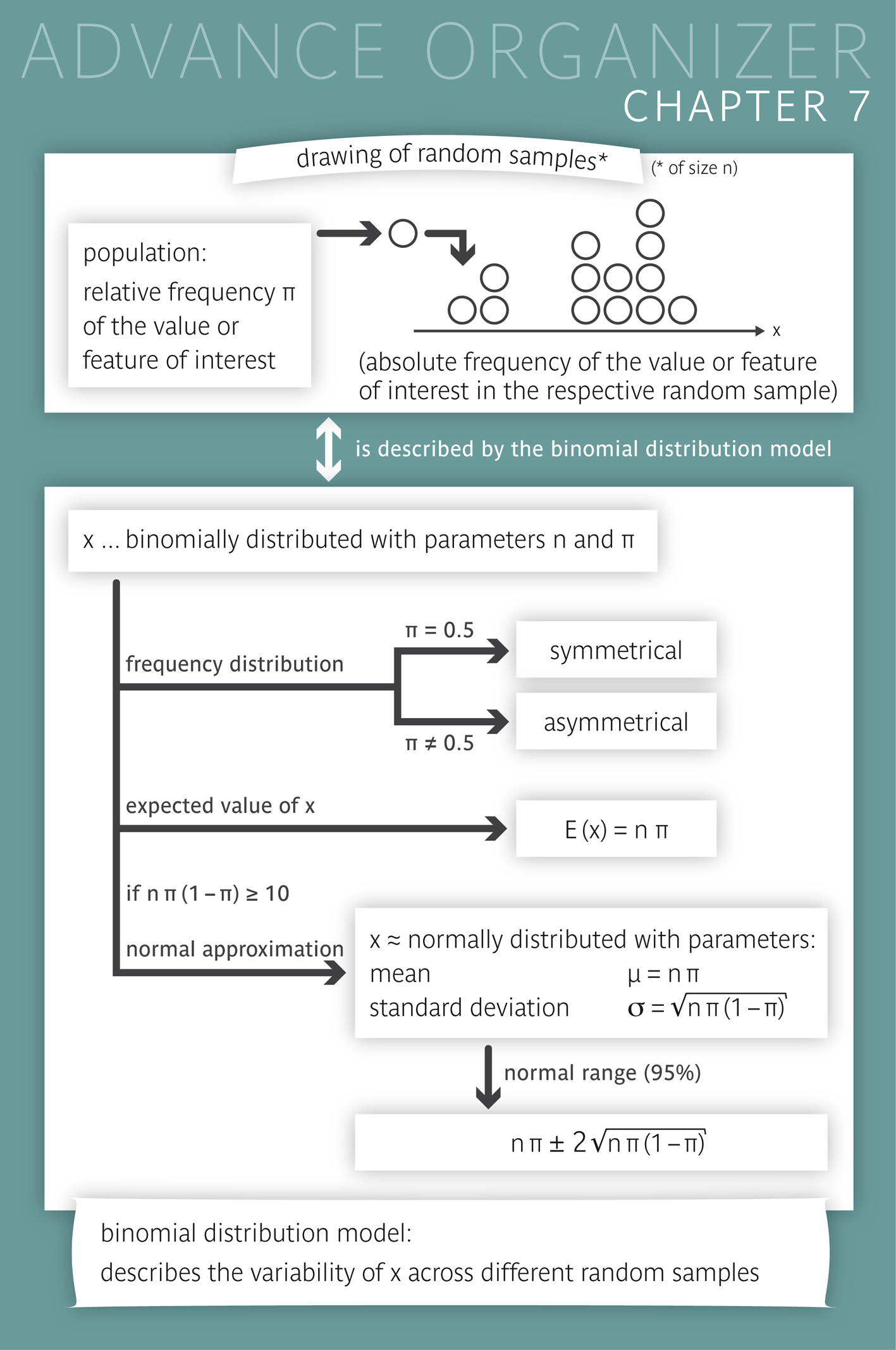
Epidemiological studies often involve the estimation of the frequency of a specific characteristic in a population. In such cases, a random sample of a certain size \(n\) is drawn from this population, and one counts how often the respective characteristic occurs in the sample (absolute frequency or count). Due to chance, this number - we denote it by \( X \) - can take various values. Most likely, we would get a different count in a second sample.

If the sample only represents a tiny fraction of the population, the probability pattern of the various possible values of \(X\) can be described by the "binomial distribution" with the parameters \(n\) (sample size) and \( \pi \) (relative frequency of the respective characteristic in the population).

In the preceding examples of tossing "heads" and throwing a six, \( \pi \) had the values \( 1/2 \) and \( 1/6 \), respectively, and \( n \) was equal to \(20\) in both examples. Any random drawing of a sample element can be regarded as an individual random experiment. Note: Here, the symbol \( X \) is not used to denote a variable which is observed in randomly chosen individuals, but it denotes a sample statistic which varies between different random samples.

Work through the following three questions with the help of the applet "Binomial distribution".

Now we are interested in the average number \( \mu \) of outcomes of interest observed in a series of \( n \) independent random experiments, where the probability of the outcome of interest equals \( \pi \) in each of the experiments. Intuition tells us that \( \mu \) must be proportional to both \( n \) and \( \pi \). Hence, \( \mu = c \times n \times \pi \), for some constant number \( c \). Since \( \mu = n \), if \( \pi = 1 \), we have \( c \times n \times 1 = n \), implying that \( c = 1 \). Therefore \( \mu = n \times \pi \). The same holds true for the average number \( \mu \) of carriers of a certain characteristic in a random sample of size \( n \) from a population in which the characteristic has a relative frequency of \( \pi \).

Answer the following question without the help of the applet.

In the example of the coin tosses you saw that the binomial distribution with the parameters \( n = 20 \) and \( \pi = 0.5 \) is symmetrical. The example of die throws illustrates that this is not always the case. Here, the parameters were \( n = 20 \) and \( \pi = 1/6 \). Take a look at figure 7.5 to see this.

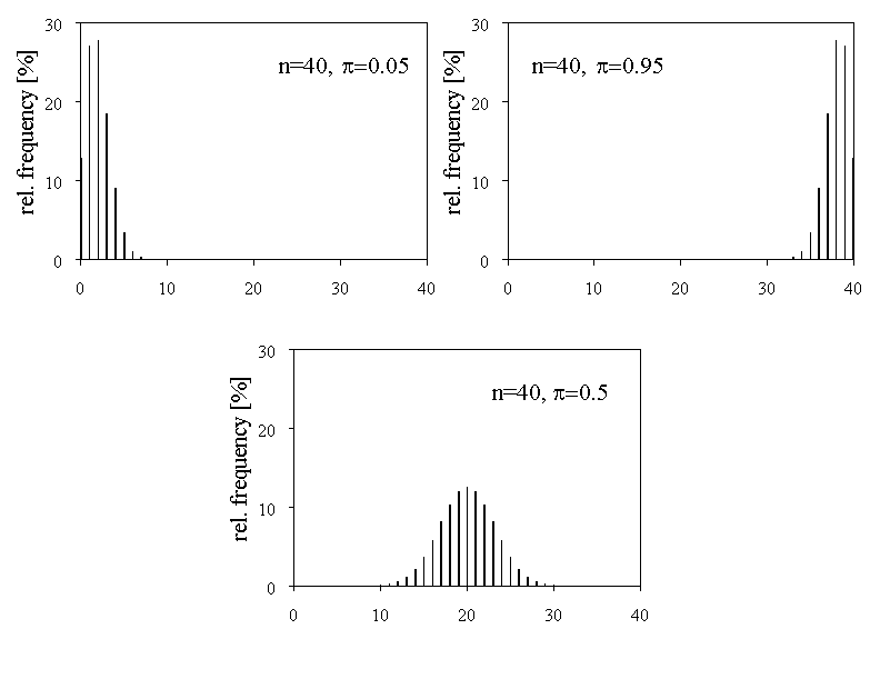
We can see that the two probability distributions with the values \( \pi = 0.05 \) and \( \pi = 0.95 \) are highly asymmetrical. For \( \pi = 0.5 \) we get a symmetrical probability distribution. In figure 7.5, \( n \) was fixed and \( \pi \) varied. But what will happen if we fix \( \pi \) and vary \( n \)? Take a look at figure 7.6 to see what happens.

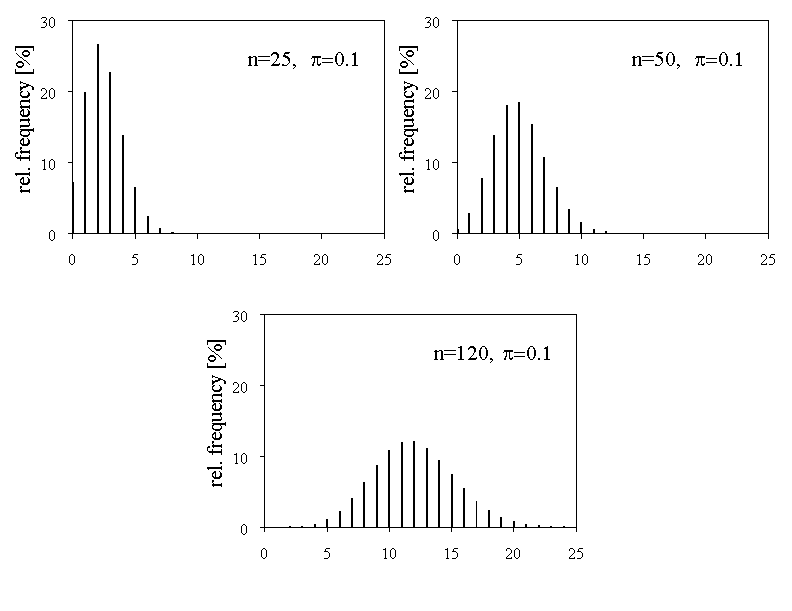
For \( n = 25 \) we get a highly asymmetrical probability distribution. With increasing \( n \), the probability distribution becomes more and more symmetrical. These observations are summarised in the following synopsis:

7.2. Approximation of the binomial distribution by the normal distribution

Take another look at the lower graph of figure 7.6. It is striking that the bar chart representing the probabilities of the respective binomial distribution has the same shape as a Gaussian bell curve. This suggests to draw the Gaussian bell curve which best fits the bar chart. We shall now see how this can be done (thereby, we ignore that binomially distributed variables are discrete and that only continuous variables can be normally distributed).

The solution is quite simple if we remember that the normal distribution is characterised by its mean value \( \mu \) and its standard deviation \( \sigma \). If a binomial distribution with the parameters \( n \) and \( \pi \) is given, then we simply approximate it by the normal distribution, which has the same mean and the same standard deviation as the respective binomial distribution.

We have seen that the mean value of the binomial distribution equals \( \mu = n \times \pi \). Moreover, the standard deviation of the binomial distribution is \( \sqrt{n \times \pi \times (1 - \pi)} \) (you just have to believe this). We thus choose \( \mu \) and \( \sigma \) as follows: \[ \mu = n \times \pi \] and \[ \sigma = \sqrt{n \times \pi \times (1 - \pi)} \]

Now take a look at figure 7.7.

In these graphs the approximating Gaussian bell curves were laid over the bar charts of probabilities of the binomial distributions.

In the upper two graphs, the approximation is not convincing, because the respective probability distributions are asymmetrical. Notice that the approximating bell curve of the upper left graph has negative \(x\)-values.

In the left graph of the middle row, the approximation is quite good even though \( n = 40 \) is relatively small. Here, the binomial distribution is symmetrical.

If we increase the sample size to \(200\), the approximations become pretty good also for the binomial distributions with \( \pi = 0.05 \) or \( \pi = 0.95 \).

When can we consider the approximation of a binomial distribution by the corresponding normal distribution as satisfactory? A general rule says that this is the case if \[ n \times \pi \times (1 - \pi) \ge 10 \, .\] This condition is met by the middle left ( \( n = 40, \pi = 0.5 \)) and the lower right (\( n = 200, \pi = 0.5 \)) distribution. The condition is clearly not met by the two upper distributions with \( n \times \pi \times (1 - \pi) = 40 \times \ 0.05 \times 0.95 = 1.9 \). In the remaining cases, where we found the approximations to be pretty good, \( n \times \pi \times (1 - \pi) = 200 \times \ 0.05 \times 0.95 = 9.5 \). Thus, the condition is almost met in these two cases.

If the variable \( X \) has a normal distribution with mean \( \mu \) and standard deviation \( \sigma \) , then the probability that \( X \) lies in the interval \( [ \mu - 2 \times \sigma, \, \mu + 2 \times \sigma ] \) is approximately \(0.95\) (chapter 6).

If \( X \) has a binomial distribution with parameters \( n \) and \( \pi \) satisfying \( n \times \pi \times (1 - \pi) \ge 10 \) , then we can consider \( X \) to be approximately normally distributed with a mean value of \( n \times \pi \) and a standard deviation of \( \sqrt{ n \times \pi \times (1 - \pi) } \).

From this we can infer that \( X \) takes a value in the interval \[ [ n \times \pi - 2 \times \sqrt{ n \times \pi \times (1 - \pi) }, \, n \times \pi + 2 \times \sqrt{ n \times \pi \times (1 - \pi) } ] \] with a probability of about \(95\%\).

7.3. The Poisson distribution

If we let \( n \) increase and \( \pi \) decrease simultaneously in a binomial distribution, while keeping the product \( n \times \pi \) constant, then a so-called Poisson distribution results in the limit. The expected value \( n \times \pi \) of the number of events of interest is usually denoted by \( \lambda \) in a Poisson distribution.

If we consider \( \lambda = n \times \pi \) as constant, then \( \pi = \lambda/n \) must hold. Hence \( \pi \) approaches \(0\) with increasing \( n \). Based on the formula of the normal distribution approximation of a binomially distributed variable \( X \), we can see that the standard deviation \(\sigma\) of \(X\) satisfies \[ \sigma = \sqrt{ n \times \pi \times (1 - \pi) } \approx \sqrt{ n \times \pi } = \sqrt{\lambda} \] if \( \pi \) is very small. Thus, the standard deviation \(\sigma\) of a variable \( X \) with a Poisson-distribution and an expected value \( E(X) = \lambda \) equals \[ \sigma = \sqrt{\lambda} \, .\]

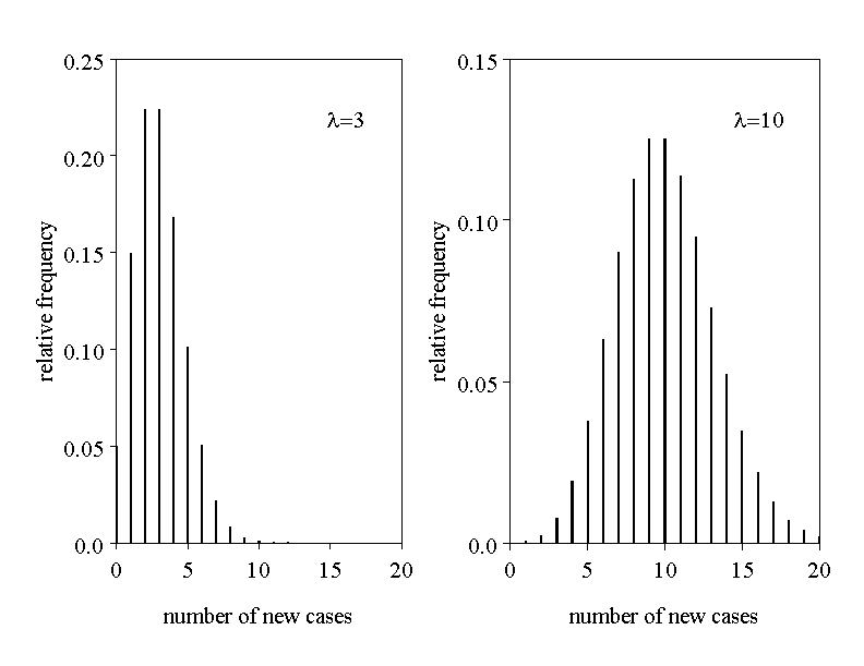
Therefore, the normal distribution approximating the Poisson-distribution with parameter \( \lambda \) has a mean value of \( \lambda \) and a standard deviation of \( \sqrt{\lambda} \). In analogy to the binomial distribution, this approximation is satisfactory if the expected number \( \lambda \) of events of interest is at least \(10\) (cf. figure 7.8).

Among other, the Poisson distribution is suitable for describing the number of occurrences of a rare event (e.g., of a rare disease) in a specific population during a certain period of time (e.g. during one year). However, for such counts to follow a Poisson distribution across several identical time intervals, the population itself and the conditions surrounding it must remain stable. Otherwise, \(\lambda\) may change over time.

One can often assume that the expected value \( \lambda \) is proportional to the length of the observation period. Figure 7.8. illustrates two such situations.

With the applet "Poisson distribution" you can generate such probability distributions for arbitrary parameter values \( \lambda \).

7.4. Summary

If we repeatedly draw random samples of size \(n\) from a population and count the number of observational units with a certain characteristic each time, then these counts are binomially distributed with parameters \(n\) and \( \pi \) (where \( \pi \) is the probability or relative frequency of the characteristic in the population).

The histogram of probabilities of the binomial distribution is symmetrical if \( \pi = 0.5 \), independent of the sample size \( n \), while it is highly asymmetrical for small to moderate sample sizes, if \( \pi \) is close to \(1\) or \(0\). The mean value of the observed counts in a series of such samples approaches the value \( n \times \pi \), the so-called expected value, if the number of samples increases.

If \( n \times \pi \times (1 - \pi) \geq 10 \), then the distribution of these counts can be considered as approximately normal, with a mean value of \( n \times \pi \) and a standard deviation of \( \sqrt{ n \times \pi \times (1 - \pi)} \). In this case, we can expect that the absolute frequency (count) of the characteristic of interest in a random sample of size \(n\) will lie in the interval \( n \times \pi \pm 2 \times \sqrt{ n \times \pi \times (1 - \pi)} \) with a probability of approx. \(95\%\).

The Poisson distribution can be considered as an "extreme case" of a binomial distribution where \( \pi \) is very small and \( n \) very large. The expectation \(E(X) = n \times \pi\) is denoted by \(\lambda\). The Poisson distribution is completely defined by this parameter \(\lambda\).

The mean value and standard deviation of a variable \(X\) with a Poisson distribution are \( \lambda\) and \(\sqrt{\lambda}\), respectively.

If \(\lambda \geq 10\), then the distribution of \(X\) can be approximated by a normal distribution with \(\mu = \lambda\) and \(\sigma = \sqrt{\lambda}\).

Among other, the number of occurrences of a rare event (e.g., a rare disease) in a fixed population during separate time intervals of equal length can generally be well described by a Poisson distribution, provided that \(\lambda\) does not change over time.