| In this chapter you are introduced to the fundamental terms of statistics, as for example "population", "sample" and "variable". These fundamental terms are the basic elements of the language of statistics, they are indispensable for the comprehension and wording of statistical problems and for the application of statistical methods. |
|
|
Educational objectives
After having worked through this chapter you will know the fundamental terms of statistics. You will be able to describe the population from which a sample was drawn and the observational units and variables involved in a sample. You can classify variables based on their values. Key words: population, sample, observational unit, variable, value, type of variable |
| A chemical company in Basel asks its employees to undergo a medical examination every five years. It has closed contracts with \(26\) medical practitioners, who agreed to examine the patients at a fixed rate paid by the company. The employees are randomly allocated to the medical practitioners. |

|
The practitioners have agreed to collect a set of basic data on the employees, including
One of these medical practitioners, Dr. Frank N. Stein, would like to get an idea of the employees' state of health himself. He decides to describe and summarize the data of his allocated patients with the help of statistics. First of all, this requires a list of the variables and of the values these variables take in each of the observational units. But what do the terms "observational unit", "variable" and "value" mean?
In the following, the term "patient file" will be used for the data of the chemical company employees, who were allocated to Dr. Frank N. Stein. In this case, the patients are the observational units. In general, subjects or objects on which data are collected are called "observational units". Depending on the research question, observational units can be persons, objects or also abstract entities (e.g., time intervals).
The data of the patients, which are available in the patient file, include height, weight, age, gender, blood pressure, blood sugar, cholesterol and haemoglobin. These characteristics are called "variables" in statistics.
As its name tells, a variable must have more than one possible value. For instance, "female" and "male" are the values of the variable "gender". Moreover, alcohol consumption of the chemical emplayees attended by Dr. Frank N. Stein is recorded using the three values (or categories) "daily", "weekly" and "seldom/never".
Caution: In common language, the statement "she/he has blue eyes" is often interpreted as a person's characteristic. However, in statistics, "blue eyes" is the value of the variable or characteristic "eye colour" in these persons. The terms "variable" (or "characteristic") and "value" (or "category") must not be confounded with each other in statistics!
In general, the totality of all potential observational units, on which one would like to collect information, is called "population". The definition of a population must be delimited in time and space and by factual conditions, and it depends on the question of interest.
For instance, the population of chemical employees from which the patients of Dr. Frank N. Stein were selected is constrained by the fact that
If we assess the variables of interest in all units of a population, we speak of a "census".
In most cases, it is not possible or not justifiable to carry out a census. Instead, a subset of observational units is selected from the respective population. Such subsets are called "samples". They should ideally consist of observational units which were randomly drawn from the population.
The terms "randomness" and "randomly" will repeatedly appear in the following sections and chapters, because they are a central element of statistics. They will be defined in more detail in chapter 4. Since randomness is omnipresent in our lives, we all have our own concept of it, which reflects our individual experiences. We regard things as being random if we cannot predict them.
When being confronted with random phenomena, we try to anticipate their various possible outcomes. At best, however, we know how frequently, resp. with which probability each of these outcomes occurs. This is why we can never predict if a coin falls on heads or tails, but we can assume that both outcomes are equally likely, i.e., that they appear equally often, on average.
Neither can we predict which individuals will be included in a random sample. However, we can perform the selection procedure in such a way that each individual of the population has the same chance to be included in the sample.
Unfortunately, the ideal case of a random sample is rarely possible in Medicine. In most cases, it is not possible to randomly select subjects from a registry covering an entire patient population. Medical studies are often based on so-called "convenience samples", which may consist of patients being examined during a certain time period.
| Term | Definion |
|---|---|
| population | the totality of all potential observational units of interest |
| sample | (random) selection of observational units from the population | observational unit | single subject, object or entity, on which data are collected |
| variable | variable or characteristic of interest, which is measured or observed in observational units |
| values | the possible values of a variable or categories of a characteristic |
If we take a look at the variables gender, alcohol consumption and body height of Dr. Frank N. Stein's data set, we immediately notice differences. Gender and alcohol consumption both have a limited number of values, but the values of alcohol consumption, i.e., "daily", "weekly" and "seldom/never" have an inherent natural order.
On the other hand, body height can take on any value between, let's say, \(100\) and \(220\) cm (in rare cases values outside this range can be observed). In principle, body height can thus take on an infinite number of values. Variables can thus be divided into different categories or data types.
Variables such as gender and alcohol consumption in Dr. Frank N. Stein's data set represent qualitative data. The values of gender have no quantitative aspect at all, and those of alcohol consumption do not represent specific quantities (even though they refer to the frequency of alcohol consumption). Qualitative data can additionally be divided into nominal and ordinal data. Instead of qualitative variables, we can also speak of "categorical variables".
If the categories defined by the values of a qualitative variable have no inherent natural order (e.g., from lower to higher or from worse to better), the variable is said to be "nominal". Gender, nationality or religion are examples of nominal variables.
Numbers are often allocated to the values of nominal variables for coding purposes (e.g., to save space). However, no meaningful calculations can be made with these numbers. For instance, if we allocate \(1\) to "male" and \(2\) to "female", how should \(2 - 1 = 1\) be interpreted in a meaningful way?
Ordinal variables take values which can be brought into a meaningful natural order, as is the case with the variable alcohol consumption with the values "daily", "weekly" and "seldom/never". In Medicine, variables like the stage of a disease or the perception of pain (with different pre-defined levels of intensity) are ordinal.
Numbers are also allocated to the values of ordinal variables for coding purposes, and it is obvious that the numbers must then reflect the order between the categories (e.g., \(1\) for "seldom/never", \(2\) for "weekly" and \(3\) for "daily" in the variable "alcohol consumption"). In general, differences between these numbers have no meaningful interpretation either.
For a variable to be quantitative, its values must be of a numerical nature. Examples of quantitative variables are body height, age or the number of children in a family. Quantitative variables are divided into discrete and continuous variables.
Discrete quantitative variables only take certain numerical values. For example the variable "number of children in a household" can only take the values \(0, 1, 2, ...,\) etc. (notice that the observational units are households in this case). Other examples are the number of physician's visits in the last \(12\) months or the number of healthy teeth if the observational units are persons. The values of quantitative discrete variables are typically assessed by counting.
In general variables which only possess a finite number of values are called discrete. This is why basically all qualitative variables are discrete. The so-called "Visual Analogue Scales" are an exception and will be shortly introduced at the end of this chapter.
Variables are called "continuous" if their values can, in principle, be measured at any degree of accuracy. A typical example of a continuous variable is body height, which could be measured with increasing accuracy in \(cm\), \(mm\), \(\mu m\), ... . The values of continuous variables are always obtained by measurements.
When analysing and interpreting data, discrete variables with a large number of values are often treated as if they were continuous (e.g. the number of leukocytes).
With continuous data, we additionally distinguish between interval- and rational-scaled variables. Body temperature is a typical example of an interval-scaled variable, as it has no meaningful zero-point, and ratios between body temperatures (e.g., \(38^{\circ} / 37^{\circ} = 1.027\)) cannot be interpreted meaningfully. A typical rational-scaled variable is body height. In this case we have an absolute zero-point and ratios can be interpreted. For instance, if a child has grown from \(1.6 m\) to \(1.7 m\) in one year, the ratio equals \(1.7/1.6 = 1.0625\) and one can say that the child's height increased by \(6.25\%\).
| Type | Definition |
|---|---|
| nominal (qualitative) | Values of nominal variables define categories without a natural order | ordinal (qualitative) | Yalues of ordinal variables define categories with a natural order |
| discrete quantitative | values of discrete quantitative variables have a quantitative meaning and their number is finite. |
| continuous (quantitative) | Values of continuous variables can, in principle, take any value in a given interval on a numerical scale |
You may now first open the applet "Grouping variables 1" and then the applet "Grouping variables 2" to test whether you are able to assign variables correctly to the four different types.
Applet "Grouping variables 1"
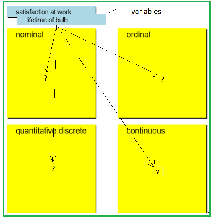
Applet "Grouping variables 2"
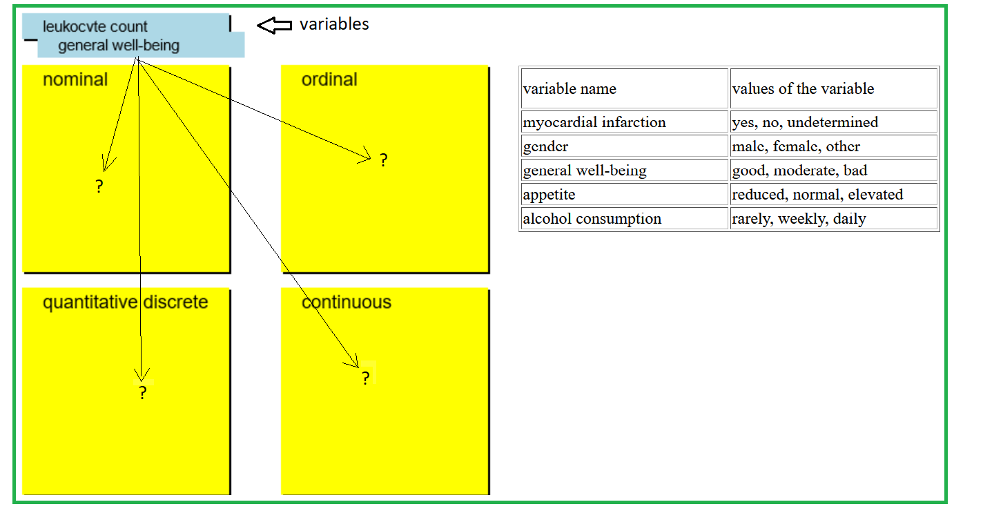
| variable name | values of the variable |
| myocardial infarction | yes, no, undetermined |
| gender | male, female, other |
| general well-being | good, moderate, bad |
| appetite | reduced, normal, elevated |
| alcohol consumption | rarely, weekly, daily |
In the past decades, so-called "Visual Analogue Scales" (VAS) have become very important. A patient can e.g. record his/her present level of pain as a specific point on a visual analogue scale whose endpoints represent the extreme values (e.g. \(0\) = complete absence of pain, \(100\) = maximum level of pain). Such scales belong to the category of ordinal variables, but are often treated like quantitative data in statistical analyses.
Every hospital doctor is familiar with the dolometer, on which a patient can indicate his/her pain level,
using a flexible line, so that the practitioner can read the respective numerical value on the back side, which is invisible to the patient.

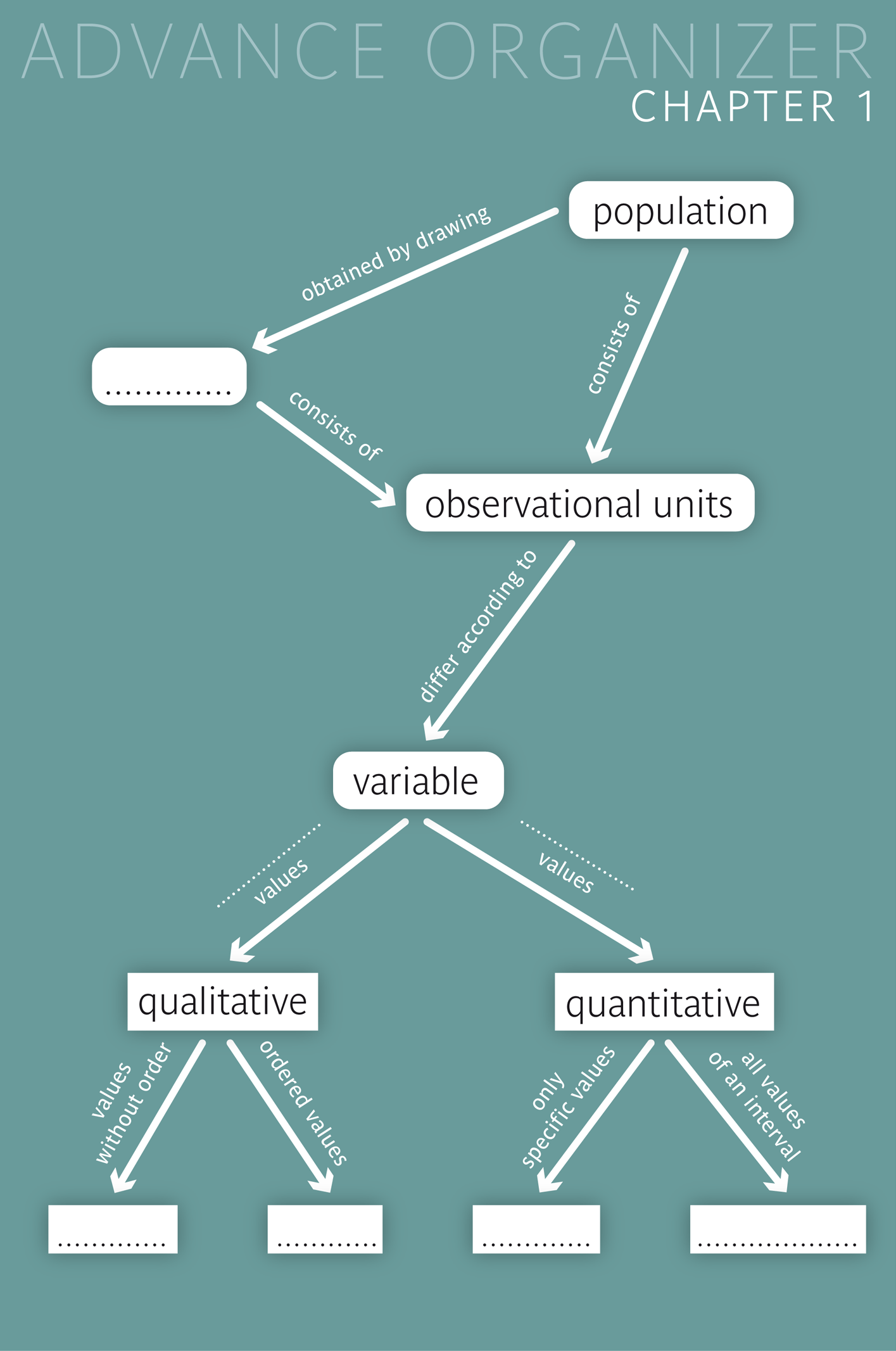
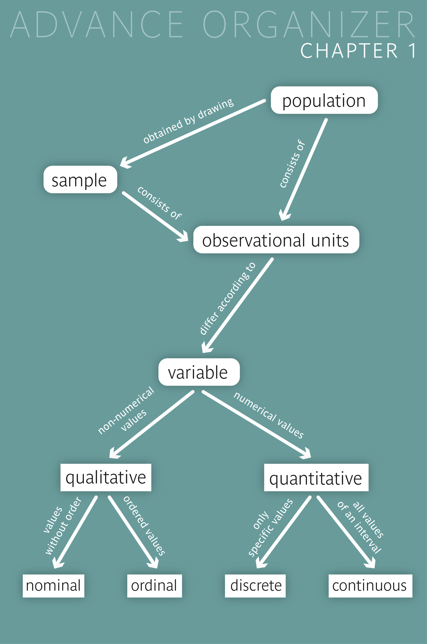
The population consists of all potential observational units, on which one would like to make a statement.
A sample is a selection of observational units from the population. Ideally, the observational units of a sample are drawn randomly. If each individual of the population has the same chance of being drawn into the sample, we speak of a simple random sample.
A variable is a characteristic, which is measured or observed on observational units. Variables whose values have no quantitative meaning are called qualitative variables, and variables whose values represent quantities are called quantitative variables.
Qualitative variables are sub-divided into nominal and ordinal variables: the values of ordinal variables have an inherent natural order, while those of nominal variables do not.
Quantitative variables are sub-divided into discrete and continuous variables: while discrete quantitative variable can only take specific numerical varlues (e.g., counts), continuous variables can, in principle, take any value of a numerical interval.