
|
We know the past but not the future! Before the calculus of probability and statistics were developed, one had to rely on subjective judgments, myths and oracles in order to estimate the probability of future events. The calculus of probability and statistics enable quantifying the likelihood of future events. |
|
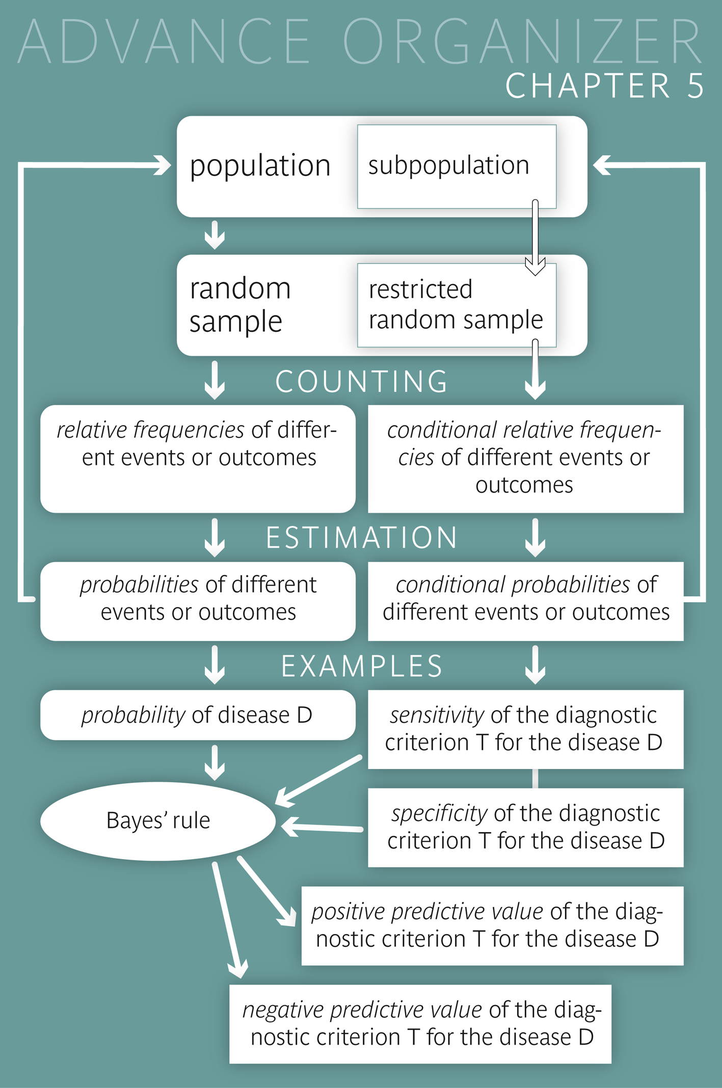
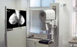
Educational objectives After having worked through this chapter you can estimate the probability of certain diseases or examination results among the subjects of a given population, based on the data of a random sample. you are familiar with the term "conditional probability" and you can explain it in your own words in concrete examples. you know the most important measures of quality and of predictive value of a diagnostic criterion or prognostic factor, and you can paraphrase them in your own words and interpret them correctly in concrete examples. you can calculate the positive and the negative predictive value of a diagnostic criterion or prognostic factor for a disease, based on the sensitivity and specificity of the criterion and the frequency of the disease. You can describe the influence of these three parameters on the predictive values. Key words: probability, two by two table, event, diagnostic criterion, prognostic factor, conditional probability, sensitivity, specificity, positive predictive value, negative predictive value, dependent and independent events or variables Previous knowledge: relative frequency (chap. 2), estimation of a population parameter (chap. 4) Central questions : What is the risk that breast cancer in an early stage cannot be detected in a mammography screening? How likely is an all-clear after further examinations following a positive mammography result? How does this likelihood change in women with a family history of breast cancer? |
The results of an American study on the diagnostic value of mammography screening are summarised in the two by two table below.
Two variables (mammography findings and breast cancer diagnosis) with their respective values (positive vs. negative and diagnosed vs. not diagnosed) are listed:
| Mammography result | Breast cancer diagnosis | Total | |
|---|---|---|---|
| diagnosed* | not diagnosed* | ||
| Positive | 132 | 983 | 1115 |
| Negative | 45 | 63650 | 63695 |
| Total | 177 | 64633 | 64810 |
We can see that 1115 of the 64810 tested women had a positive result in the mammography screening. This corresponds to a relative frequency of \(1115/64810 = 0.0172\) or \(1.72\%\). The probability that a mammography in randomly selected woman of the population results in a positive outcome can thus be estimated at \(0.0172\) or \(1.72\%\). (The difference between an estimated value and the real value of a population parameter was treated in chapter 4.)
Moreover, the probability of a diagnosis of breast cancer can be estimated at \(177 / 64818 = 0.0027\) or \(0.27\%\)) for a randomly selected woman who would be examined for breast cancer.
|
Definition 5.1.1
The probability of a randomly chosen observational unit to show a specific characteristic is equal to the relative frequency of this characteristic in the underlying population. |
|
Synopsis 5.1.1
Probabilities (at a population level) can be estimated by the corresponding relative frequencies in a random sample from the respective population. |
Probabilities always relate to events \(E\) of which we do not know if they will occur or not (e.g. the occurrence of a specific disease \(D\), a positive result of a diagnostic test, etc.).
Here, the term "event" has a wider meaning than in common language. It does not only refer to something that may or may not happen, but it can also be used for the ascertainment of a specific characteristic in a randomly selected person (e.g., that this person is female).
The probability \(P(E)\) of an event \(E\) indicates the level of certainty with which it can be expected. (The symbol \(P\) is the first letter of the Latin word "probabilitas".)
This leads us to the following alternative definition of probability.
|
Definition 5.1.2
The probability of an event describes the level of certainty with which it can be expected (\(1\) = "one can be absolutely certain that the outcome will occur", \(0\) = "one can be absolutely certain that the outcome will not occur") |
The non-occurrence of an event \(E\) also represents an event. This event, which is complementary to \(E\) is denoted \( E^c \). As one either observes \(E\) or \( E^c \), the following equation holds \[ P(E) + P(E^c) = 1 .\] Hence, the two probabilities are related by the following equation \[ P(E^c) = 1 - P(E) \]
Without the knowledge of the mammography findings, only one probability value (\(P(E) = 0.0027\)) can be attached to the potential presence of breast cancer in a given woman. However, if we know her mammography result, we can allocate her to a more narrowly defined population. As a consequence, the probability of the disease changes: it increases for women with a positive mammography result, and it decreases for women with a negative result.
|
Definition 5.2.1
If the probability of an event \( E_2 \) is calculated under the condition \( E_1 \), we speak of a "conditional probability". In this case, the population is restricted by condition \( E_1 \). The notation for a conditional probability is \( P(E_2|E_1) \) ("probability of \(E_2\) given \(E_1\)"). |
In our example, we get estimates of conditional probabilities by confining ourselves to a specific line or a specific column of the two by two table. For instance, the probability of a breast cancer diagnosis (\( E_2 \)) after a positive result of the mammography (\( E_1 \)) can be estimated at \(132/1115 = 0.1184\) or \(11.8\%\), according to the first line of the two by two table. The population of interest now consists of the women with a positive mammography result. This special conditional probability defines the "positive predictive value" of mammography screening.
If a woman has received a negative mammography result ( \( \rightarrow \) second line of the two by two table), the probability of her being diagnosed with breast cancer within a year is much smaller, namely approximately \(45 / 63695 = 0.0007\) or \(0.07\%\). Hence the probability that a woman with a negative mammography result will not be diagnosed with breast cancer within a year can be estimated at \( 1 - 0.0007 = 0.9993\) or \(99.93\%\). This conditional probability is referred to as "negative predictive value".
Other important examples of conditional probabilities are the "sensitivity" and the "specificity" of a diagnostic criterion or prognostic factor. The sensitivity tells how reliably the criterion resp. factor can detect or predict the respective disease and the specificity tells how safely the absence of the criterion resp. factor can predict the absence of the disease. Unlike the predictive values, neither the sensitivity nor the specificity are influenced by the frequency of the disease and hence both of them provide context-independent quality measures of the respective criterion or factor.
| Definition 5.2.2 | |
| Measures of quality: | |
| Sensitivity of a criterion for a disease |
Probability of the criterion being fulfilled in
a person with the respective disease = "Proportion of the positively tested among those with the disease" |
| Specificity of a criterion for a disease |
Probability of the criterion not being fulfilled in
a person without the respective disease = "Proportion of the negatively tested among those without the disease" |
| Definition 5.2.3 | |
| Measures of the predictive value: | |
| Positive predictive value (PPV) of a criterion for a disease |
Probability of a person carrying
the respective disease (or getting it later), if the criterion is fulfilled = "Proportion of persons with the disease among those fulfilling the criterion" |
| Negative predictive value (NPV) of a criterion for a disease |
Probability of a person not carrying the disease (or not getting it later),
if the criterion is not fulfilled. = "Proportion of persons without the disease among those not fulfilling the criterion" |
Here, the term "criterion" is used for a diagnostic test or criterion or for a prognostic factor.
If we are talking about a prognostic factor \(F\) for a disease \(D\), then its sensitivity and specificity can be estimated from a "retrospective" study (or case-control study). In such a study, people with the disease \(D\) are compared to people without the disease regarding the relative frequency of \(F\). Apart from the presence resp. absence of the disases, the two groups should be as similar as possible. Here, one estimates the conditional probabilities \[ \begin{aligned} P(F|D) & = \text{Probability that a person with the disease D showed factor F} \\ & = \text{Sensitivity of F for D} \end{aligned} \] and \[ \begin{aligned} P(F|D^c) & = \text{Probability that a person without the disease D showed factor F} \\ & = 1 - \text{specificity of F for D}. \end{aligned} \] Conversely, we can compare a group of people in whom factor \(F\) is present and a group of people without factor \(F\) with respect to the frequency of a later occurrence of \(D\) in a "prospective" study. Apart from the presence resp. absence of \(F\), the two groups should be as similar as possible at the beginning. Here, one estimates the conditional probabilities \[ \begin{aligned} P(D|F) & = \text{Probability that a person with factor F gets the disease D} \\ & = \text{positive predictive value of F for D} \end{aligned} \] and \[ \begin{aligned} P(D|F^c) & = \text{Probability that a person without factor F gets the disease D} \\ & = 1 - \text{negative predictive value of F for D}. \end{aligned} \]
We want to examine if there is an association between the age of the mother and the weight of her child at birth. For this purpose, we distinguish if the mother is younger or older than 20 years and if the baby weighs more or less than 2500 g. Two different approaches are possible.
Retrospective study: The populations are defined by the event of interest, namely if the weight of the baby at birth is lower or higher than 2500 g. We draw a sample from each of these populations, e.g., 1000 babies who weigh less than 2500 g and 1000 babies who weigh more than 2500 g and examine the age of the mothers. Based on the observed frequencies, the respective conditional probabilities can be estimated. If the proportion of young mothers were clearly higher among the mothers with low weight babies compared to the mothers with "normal" weight babies, this would provide evidence for an increased risk of giving birth to a low weight baby among women under the age of 20 years.
Prospective study: The populations are defined by the factor of interest, namely the age of the mother. One sample is drawn from each of the two populations, e.g. 1000 mothers who are younger than and 1000 mothers who are older than 20 years, and then we observe the weight of their children at birth. If the proportion of lower weight babies were clearly higher among young mothers as compared to older mothers, this would provide evidence for an increased risk of giving birth to a low weight baby among women under the age of 20 years.
Two events \( E_1 \) and \( E_2 \) are called "independent", if the probability of \( E_1 \) does not change if we know that \( E_2 \) has occurred and vice versa, i.e. if the following applies: \[ P(E_1|E_2) = P(E_1) \,\, \text{and} \,\, P(E_2|E_1) = P(E_2) \, .\] For example the events \( E_1 \) = "Mister A was diagnosed with diabetes" and \( E_2 \) = "Mister B was not diagnosed with diabetes" are independent of one another, if the two men are randomly chosen from a population. The events "Person X has blood group 0" and "Person X is female" are also independent from one another, if person X was randomly chosen. However, as a general rule, events \( E_1 \) and \( E_2 \) concerning the same person are not independent. This also applies to events concerning two persons who are somehow related.
|
Definition 5.3.1
Two events \( E_1 \) and \( E_2 \) are said to be "independent", if \[ P(E_2|E_1) = P(E_2) \,\, \text{and} \,\, P(E_1|E_2) = P(E_1) ,\] i.e. if the two events do not contain any information about each other. However, if \[ P(E_2|E_1) \neq P(E_2) \,\, \text{and} \,\, P(E_1|E_2) \neq P(E_1) , \] the two events \( E_1 \) and \( E_2 \) are dependent. |
The probability that both \( E_1 \) and \( E_2 \) occur is denoted \( P(E_1 \cap E_2) \). (In set theory, the sympbol \( \cap \) denotes the intersection of two sets, and we may interpret \( E_1 \cap E_2 \) as the intersection of the two events \( E_1 \) and \( E_2 \)).
The following applies \[ \begin{aligned} P(E_1 \cap E_2) & = P(E_1) \times P(E_2|E_1) \\ & = P(E_2) \times P(E_1|E_2) \end{aligned} \]
For instance, the probability that a woman has a positive mammography result but will not be diagnosed with breast cancer within the following year can be calculated (or estimated) as follows: \[ \begin{aligned} P(\text{pos. mammography result} \cap \text{no breast cancer diagnosis}) & = P(\text{pos. mammography result}) \times P(\text{no breast cancer diagnosis| pos. mammography result}) \\ & = 0.017 \times (1 - \text{positive predictive value}) \\ & = 0.017 \times (1 - 0.118) \\ & = 0.017 \times 0.882 \\ & = 0.015 \end{aligned} \]
To get from the first to the second equation, we have used the fact that the formula for the probability of a complementary event also applies if the probabilities are conditional: \[ P(E_2^c|E_1) = 1 - P(E_2|E_1) \]
As an explanation of the product formula cited above we can take a look at the following schematic two by two table.
| \( E_2 \) | \( E_2^c \) | Total | |
| \( E_1 \) | a | b | a+b |
| \( E_1^c \) | c | d | c+d |
| Total | a+c | b+d | a+b+c+d |
The following probabilities can be estimated based on this table. \[ \begin{aligned} & P(E_1) = \frac{a + b}{a + b + c + d} \\ & P(E_2) = \frac{a + c}{a + b + c + d} \\ & P(E_1|E_2) = \frac{a}{a + c} \\ & P(E_2|E_1) = \frac{a}{a + b} \\ & P(E_1 \cap E_2) = \frac{a}{a + b + c + d} \end{aligned} \] Multiplying the last fraction with \( \frac{a+b}{a+b} \) we get: \[ P(E_1 \cap E_2) = \frac{a}{a+b+c+d} = \frac{a+b}{a+b+c+d} \times \frac{a}{a+b} = P(E_1) \times P(E_2|E_1) \] and multiplying it by \( \frac{a+c}{a+c} \) , we get \[ P(E_1 \cap E_2) = \frac{a}{a+b+c+d} = \frac{a+c}{a+b+c+d} \times \frac{a}{a+c} = P(E_2) \times P(E_1|E_2) \]
If the two events \( E_1 \) and \( E_2 \) are independent, the product formula can be simplified as follows \[ P(E_1 \cap E_2) = P(E_1) \times P(E_2) \]
The probability that two independent events occur together is thus equal to the product of the two individual probabilities.
|
Synopsis 5.3.1
The probability that two independent events \( E_1 \) and \( E_2 \) occur together is equal to the product of the individual probabilities, i.e. \[ P(E_1 \cap E_2) = P(E_1) \times P(E_2) \, . \] If two events \( E_1 \) and \( E_2 \) are dependent of one another, the probability of their joint occurrence is given by \[ P(E_1 \cap E_2) = P(E_1) \times P(E_2|E_1) = P(E_2) \times P(E_1|E_2) \] |
We can calculate the estimate of the positive predictive value of the mammography screening for the diagnosis of breast cancer within the following year easily from the two by two table. In this chapter, you will learn how to calculate the positive predictive value of a diagnostic test or criterion, if only the relative frequency of the disease in the population of interest and the sensitivity and the specificity of the diagnostic test or criterion are known.
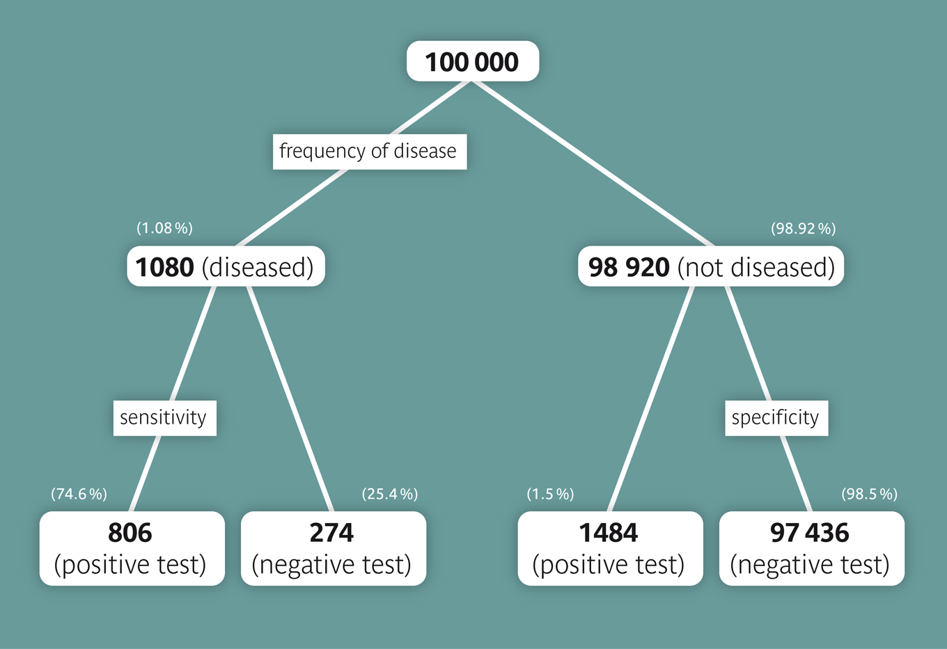
We can assume that women, whose mothers died of breast cancer, have about a fourfold risk of getting breast cancer themselves. We therefore assume that the risk to get breast cancer within one year is \( 1.08% = (4 \times 0.27%) \) for such women. We now want to calculate the positive predictive value of a positive mammography result among women, whose mothers died of breast cancer. To do so, we assume that the values of sensitivity (\(74.6 \%\)) and specificity (\(98.5 \%\)) calculated before are still valid and represent the true values in the underlying population. To simplify the task, we proceed from a collective of 100,000 women: On average, we could thus expect \( 100,000 \times 0.0108 = 1080 \) women with a diagnosis of breast cancer of which \( 1080 \times 0.746 = 806 \) would have a positive mammography result. On the other hand, of the 98920 women without breast cancer, \( 98920 \times (1 - 0.985) = 1484 \) would have a positive test result as well. On average, we could thus expect 1484 + 806 = 2290 cases with a positive mammography result, of which 806 would be confirmed with a breast cancer diagnosis. The positive predictive value would therefore be \(806/2290 = 0.352\) or \(35.2 \%\). This is not quite four times the positive predictive value among women in general, since the denominator of the ratio also increased.
According to the SCARPOL study (1992-93) [1], approx. \(9 \%\) of all children in Switzerland were diagnosed with asthma during their childhood. Since asthma is hereditary to a certain extent, we are interested in the probability of a child with an asthma diagnosis to have at least one parent with asthma. In the same study, this percentage was estimated at \(26\%\) (sensitivity of the criterion "parental asthma" for the asthma diagnosis in the child). These are more than the approx. \(18\%\), which could have been expected if asthma were not hereditary, if the frequency of asthma had been the same in the generation of parents, and if the presence of asthma in one parent were independent of the presence of asthma in the other parent. In comparison, only \(8\%\) of the children without an asthma diagnosis had at least one parent with asthma. Hence about \(92\%\) of the "healthy" children did not have the prognostic criterion "parental asthma" (specificity).
This approach can be visualized with the applet "Pre- and post-test probability" which provides a graphical representation of the Bayes-formula.
Notice that the probability of the disease \(P(D)\) is also referred to as "pre-test probability" of the disease and the positive predictive value as "post-test probability" of the disease.
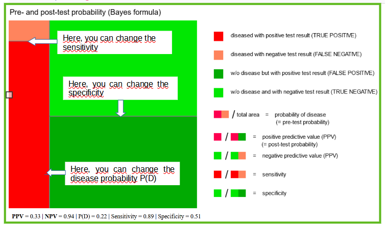
Adjust the diagram to our example. If you have placed all the lines correctly, the value of \(0.24\) which you had previously calculated should appear in the box of the positive predictive value underneath the graph.
The leading symptom of asthma is the so-called wheezing (even though there are asthmatics without this symptom). If we reinforce the condition of parental asthma by this additional condition, we can get closer to the diagnosis of asthma. Based again on the SCARPOL study, we can assume that \(92 \%\) of the diagnosed asthmatic children with at least one asthmatic parent have shown this symptom at some point of time, but that this also applies to \(30 \%\) of the children without asthma having a parent with asthma.
|
Synopsis 5.4.1
1. The positive and negative predictive values increase with increasing sensitivity of the diagnostic test or criterion (if the specificity does not decrease at the same time and the disease frequency does not change). 2. The positive and negative predictive values increase with increasing specificity of the diagnostic test or criterion (if the sensitivity does not decrease at the same time and the disease frequency does not change). 3. If the sensitivity and specificity of the diagnostic test or criterion remain unchanged, the positive predictive value increases with increasing disease frequency and decreases with decreasing disease frequency. 4. If the sensitivity and specificity of the diagnostic test or criterion remain unchanged, the negative predictive value decreases with increasing disease frequency and increases with decreasing disease frequency. Because of 3) and 4), a broad screening for a rare disease requires strong arguments. |
To conclude this section, we also give the classical Bayes' formula for the computation of the positive and negative predictive values from the pre-test probability of diseae \(P(D)\) and the positive and negative predictive values of the respective diagnostic test or criterion \(T\). The sensitivity of \(T\) for \(D\) is denoted by \(P(T+|D)\) and the specificity by \( P(T-|D^c) \).
| Syopsis 5.4.2 (Bayes' formula) \[ \begin{aligned} PPV = P(D|T+) & = \frac{P(D) \times P(T+|D) } {P(D) \times P(T+|D) + P(D^c) \times P(T+|D^c)} \\ & = \frac{P(D) \times P(T+|D)} {P(D) \times P(T+|D) + (1-P(D)) \times (1 - P(T-|D^c)} \\ & = \frac{P(D) \times \text{sensitivity}} {P(D) \times \text{sensitivity} + (1-P(D)) \times (1-\text{specificity}) } \end{aligned} \] \[ \begin{aligned} NPV = P(D^c|T-) & = \frac{P(D^c) \times P(T-|D^c)} {P(D^c) \times P(T-|D^c) + P(D) \times P(T-|D)} \\ & = \frac{(1-P(D)) \times P(T-|D^c) } {(1-P(D)) \times P(T-|D^c) + P(D) \times (1 - P(T+|D)} \\ & = \frac{(1-P(D)) \times \text{specificity}} {(1-P(D)) \times specificity + P(D) \times (1 - \text{sensitivity})} \end{aligned} \] |
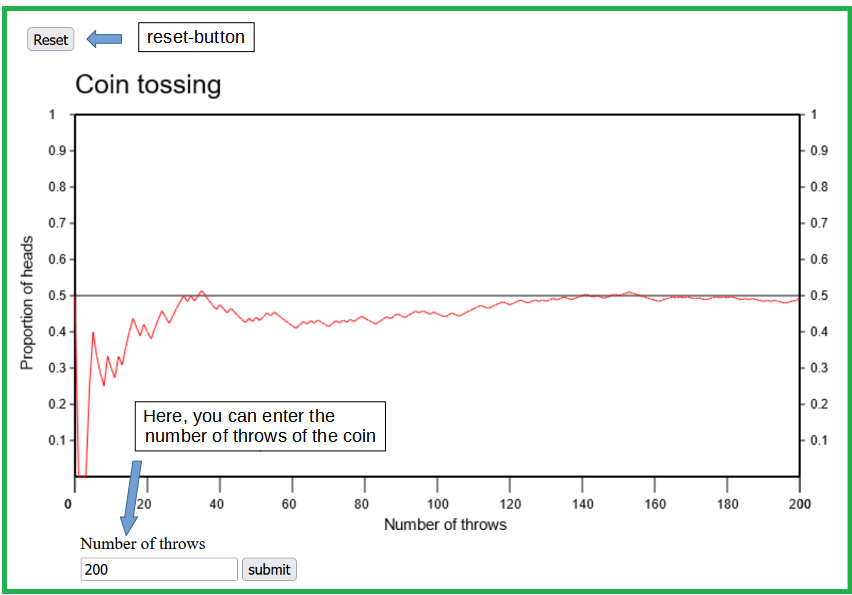
If a coin is tossed repeatedly, it shows heads or tails in a random succession. With a so-called fair coin we can expect heads and tails with equal probability at each toss. The repeated tossing of a fair coin can be simulated with the applet "Coin tossing". It illustrates the random fluctuations of the proportion of heads. These fluctuations are getting smaller and smaller as the number of coin tosses increases, up to the point at which the relative frequency levels off at a value of \(0.5\).
With a real coin, we would probably get a limit value slightly different from \(0.5\).
The probability that a toss of a specific coin shows heads equals this limit value.
Coin tossing represents a classical example of a random experiment.
Other examples of random experiments are
At first sight it may be surprising that b) and c) are also random experiments. However, the effect of a medical treatment varies randomly from patient to patient as well. Even the dose of pills shows slight random variations.
We always speak of a random experiment if the result of the underlying procedure includes a random component. Although most random experiments have a multitude of possible outcomes, the question of interest may only be whether or not the observed outcome meets certain criteria (e.g., if the health condition of a patient has improved after the treatment, if the number 13 can be found among the randomly drawn numbers, or if the dose of a pill lies within a certain tolerance margin). Events are defined by such criteria. We say that a certain event occurred if the outcome of the random experiment met the respective criterion. The probabilities of the various possible events are of primary interest in a random experiment. They are defined as follows, in analogy to the concrete example of coin tossing:
|
Definition 5.5.1
The probability that a certain event occurs in a random experiment corresponds to the limit of the relative frequency of the event in an infinitely long series of repetitions of the respective random experiment. |
We can thus only know the probabilities of the various outcomes of a random experiment by approximation (i.e., by repeating the random experiment a large number of times). Of course, it is then important that the conditions of the random experiment do not change over time.
The probability of a non-experimental event corresponds to its relative frequency in the population of interest. Such probabilities are estimated by the corresponding relative frequencies observed in random samples from the respective population.
Conditional probabilities refer to populations restricted by a condition. Important examples of conditional probabilities in Medical Science and Epidemiology are the sensitivity, the specificity, the positive predictive and the negative predictive value of a diagnostic test or criterion for a disease.
Two events are called independent, if they do not contain any information about each other. In this case, the probability of their joint occurrence is calculated as the product of the individual probabilities. Otherwise the calculation of joint probabilities involves conditional probabilities.
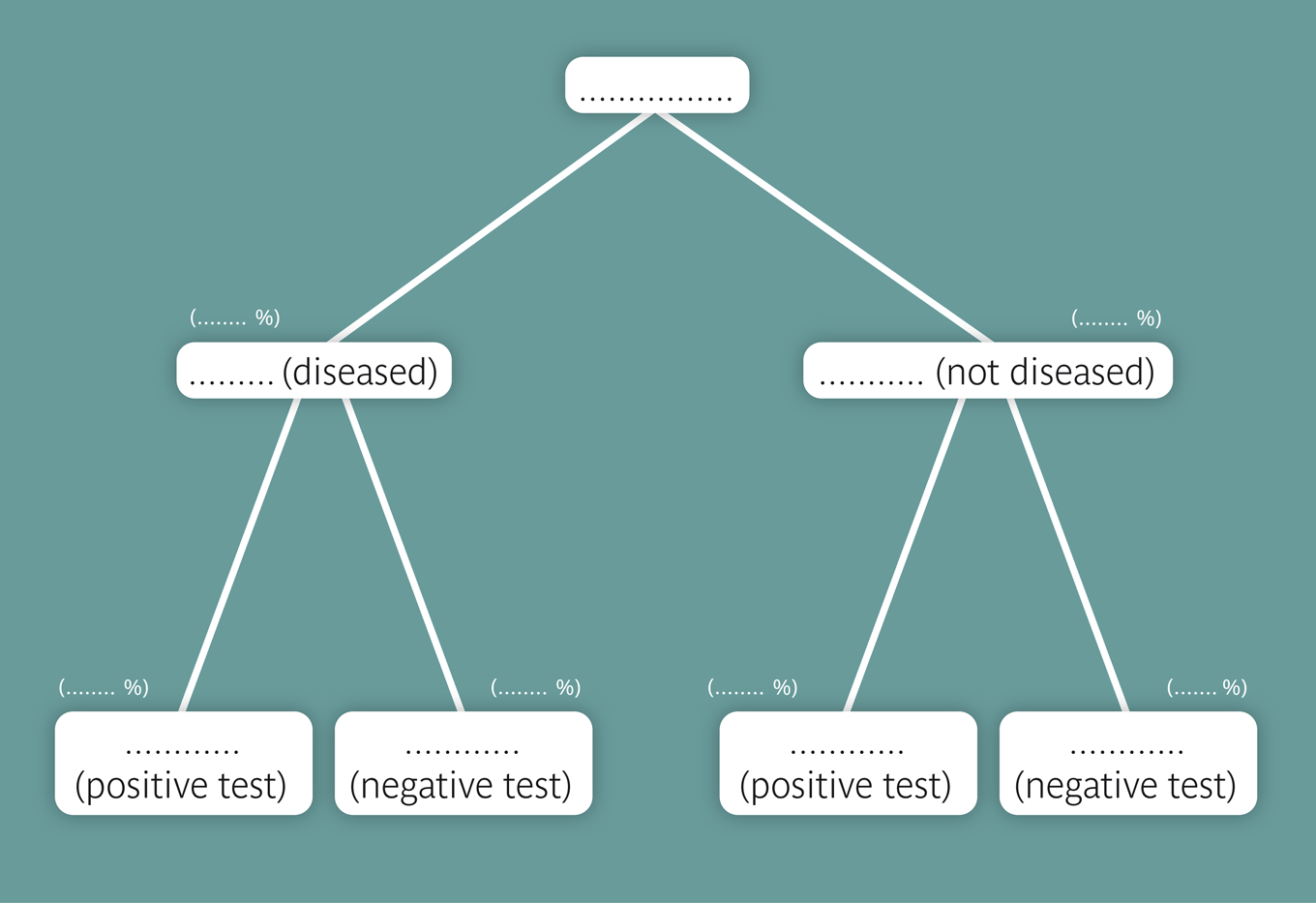
We often only know the sensitivity and the specificity of a diagnostic test or criterion and have to calculate its positive and negative predictive values as a function of the disease frequency in the underlying population. Probability trees are suitable for such calculations. The Bayes' formula captures these calculations in a compact form. It can be visualized using the Bayes applet.
The probability of a specific outcome of a random experiment can be estimated by repeating the respective experiment a large number of times and determining the relative frequency of the outcome in this experimental series.

[1] S.W. Fletcher and J.G. Elmore (2003)
Mammographic Screening for Breast Cancer
New England Journal of Medicine; 348: 1627-
[2] C. Braun-Fahrlaender, et. al. (1997)
Respiratory Health and Long-term Exposure to Air Pollutants in Swiss Schoolchildren
American Journal of Respiratory and Critical Care Medicine; 155:1042-9