
|
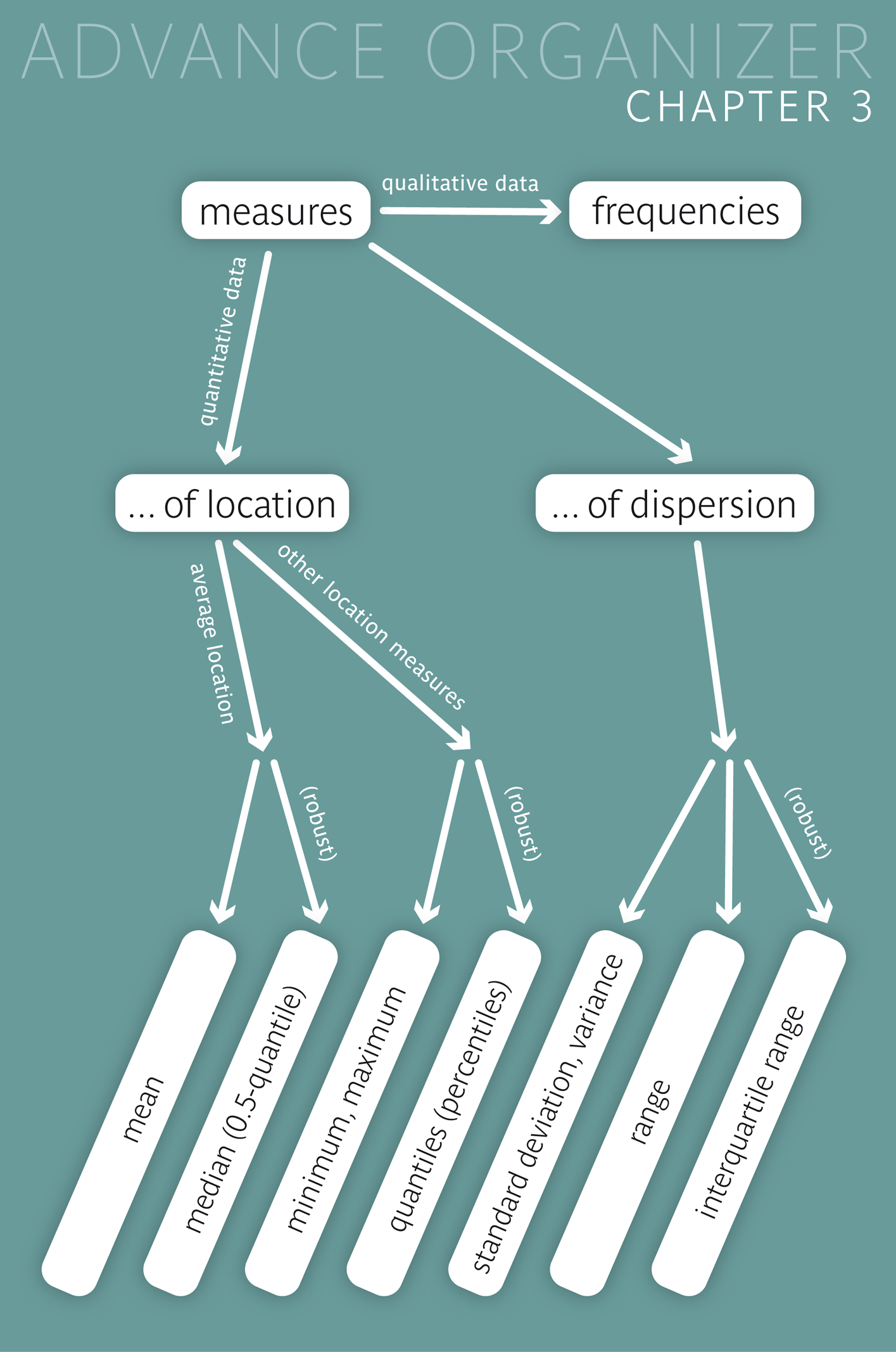
For a good description of collected data material, we also need statistical measures (or statistics) in addition to tabular and graphical representations. With these statistics, the distribution of the data, which was graphically visualised in chapter 2, can be summarised in a compact and comprehensible way by few numbers. When dealing with quantitative data, we primarily distinguish between location measures and dispersion measures. |
|
Educational objectives
After having worked through this chapter you will be familiar with different statistical measures (statistics) and their meaning, in particular you will know the difference between location measures and dispersion measures. Furthermore you can calculate statistics yourself and you can also construct and interpret a boxplot. Key words: mean value, median, quartiles, quantiles, variance, standard deviation, range, interquartile range. Previous knowledge: type of variable (chap. 1), boxplot (chap. 2) |
In the following table Dr. Frank N. Stein has listed the age of the \(18\) female chemical company employees. The \(18\) values of age are from now on represented by \(x_1, x_2, . . . , x_{18}\). Hence e. g. \(x_5 = 35\).
| Patient | Age (yr) | Patient | Age (yr) |
|---|---|---|---|
| 1 | 33 | 10 | 47 |
| 2 | 41 | 11 | 51 |
| 3 | 58 | 12 | 56 |
| 4 | 40 | 13 | 32 |
| 5 | 35 | 14 | 37 |
| 6 | 41 | 15 | 37 |
| 7 | 43 | 16 | 44 |
| 8 | 47 | 17 | 65 |
| 9 | 36 | 18 | 52 |
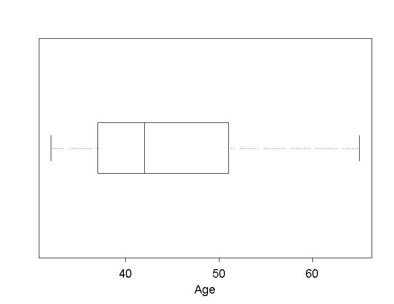
These data are visualised in the following boxplot.
Central questions:
Question: How old are Dr. Frank N. Stein's female chemical company employees?
This question can be answered by examining the individual age values. However, the table gives too many details. The goal is to get a summary of the age values using a measure of location.
Measures of location provide information on the magnitude of the collected data, i.e., on their location on the underlying numerical scale. The goal is to calculate a number which represents the data well. A measure of location gives an answer to the question "Where are the data located?". This question can be specified in different ways: `
According to the various possible questions, there are also various measures of location.
Dr. Frank N. Stein would like to find out the mean age of his female chemical company employees. To do so, he has to sum up all the age values of the \(18\) women and divide the sum by \(18\). Therefore the mean age is \[ \bar{x} = \frac{x_1 + x_2 + ... + x_{18}}{ 18} = \frac{795}{ 18} = 44.17 \, \text{years} \] The mean value is also called "arithmetic mean", "average value" or just "mean". It is usually denoted by \(\bar{x}\) (read: x bar). if the individual observations are denoted by \( x_{1}, x_{2}, ... , x_{18} \). (If the individual observations were denoted by \( y_{1}, y_{2}, ..., y_{18} \), the mean would be \(\bar{y} \).) The value of \(\bar{x} = 44.17\) is the mean age of the \(18\) women. At first sight, it may be surprising that none of the women is exactly \(44.17\) years old. But this is the normal situation with mean values.
You have certainly calculated mean values before. However, mean values are only meaningful under certain conditions.
|
Synopsis 3.1.1
A meaningful calculation of the mean value is only possible with quantitative variables, because the calculation of sums makes sense only for quantitative data. |
In this context, take a look at the following question:
The mean value is a measure of the mean location of the data. Another measure of the mean location is the "median". The idea of "mean" is conceived differently in this case. The median can be derived according to the following rule:
Find a number such that fifty per cent of the data are smaller and fifty percent larger than this number
However, such a number can only exist if the sample size is even (only an even number can be divided by \(2\) !). If the sample size is uneven, then we try to approximately fulfill this condition. In this case, the following rule is applied:
We first arrange the individual values in ascending order. Then the value which lies exactly in the middle of the ordered series is identified by counting.
What will however happen if the sample size is even, as in Dr. Frank N. Stein's 18 female patients? In this case, it is not possible to directly define the median by counting. This problem can be solved as follows:
We equate the median with the arithmetic mean of the two values lying in the center of the ordered series.
Dr. Frank N. Stein can now calculate the median of the age of his \(18\) female patients by considering the two age values which lie in the center of the ordered series \[ 32, 33, 35, 36, 37, 37, 40, 41, \boldsymbol{41}, \boldsymbol{43}, 44, 47, 47, 51, 52, 56, 58, 65 \] i.e. the \(9\)-th and the \(10\)-th value, and then calculating the arithmetic mean of these two values (i.e., \(41\) and \(43\)). In this sample, the median of age is thus \[ \tilde{x} = \frac{41 + 43}{2} = 42 \, \text{years}. \]
The median is usually denoted by \( \tilde{x} \) (read: "x tilde").
This method of determining the median corresponds to its reading from the distribution function, as it was explained in chapter 2.
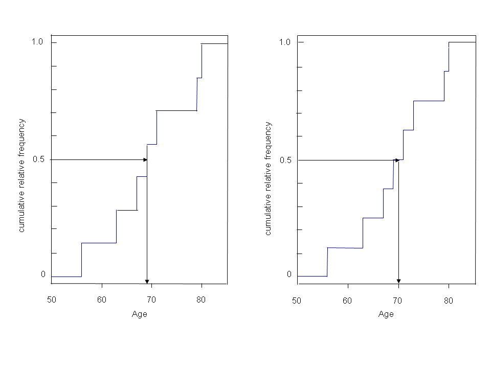
In order to determine the median of the data underlying the empirical distribution function, we read the value of age for which the distribution function has a cumulative relative frequency of \(0.5\).
If we have an uneven sample size, as in the left part of figure 3.3, then \(0.5\) marks the midpoint of a step. In this case, the median can be directly read as the x-value of this step.
If we have an even sample size, as in the right part of figure 3.3, then the step function runs horizontally at the level \(0.5\). Therefore any value of age within this horizontal line segment is a potential candidate for the median. It is thus natural to take the value of weight, which cuts this horizonal line segment in half (i.e., the arithmetic mean of the two age values limiting the segment). Since we have to calculate an arithmetic mean when determining the median of even-numbered samples, a meaningful interpretation of the median is not possible for non-quantitative variables either.
|
Synopsis 3.1.2
Equal numbers of values lie on both sides of the median. If the sample size n is even, then this can be sharpened to \(50\%\) of the data lying on either side of the median. |
The mean value and the median are both statistical measures for the mean location or the centre of the data. Therefore, the following questions arise:
In order to answer these questions, we first have to examine how strongly the mean value and the median are influenced by extreme values. Work through the following questions
Your findings are summarized in the following synopsis
|
Synopsis 3.1.3
The mean value responds very strongly to changes in the largest and smallest values of the sample, while the median is not affected by such changes. In the language of statistics, this property is referred to as "robustness" of the median. |
You can convince yourself of the robustness of the median by opening the applet "Comparison of mean value and median".
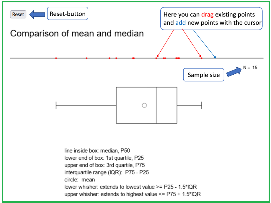
Answer the following question with the help of this applet.
You have seen that individual extreme values can strongly influence the mean. If the difference between the median and the mean is significant, this either indicates the presenece of extreme values or that the data have a skewed distribution. In such situations, the median is the more adequate measure of location. A distribution is said to be "skewed", if the spread of the values is different to the left and to the right of the median.
The decision of whether to calculate the mean or the median also depends on the underlying question. For instance, if we want to estimate the annual number of hospitalisation days from a sample of stationary stays in a county hospital, then the mean length of the hospital stays of this sample can be multiplied by the annual number of hospital stays. In this case, the mean is the right choice. However, if we are interested in a typical value, the median is more appropriate.
As Dr. Frank N. Stein is also interested in the range of age of his female patients, he wants to determine the minimum and the maximum of their ages. He will find that the smallest age value in his data set is \(x_{[1]} = 32\) years, and that the largest one is \( x_{[18]} = 65\) years. In general, the \(k\)-th value of a series of quantitative data arranged in ascending order is denoted by \( x_{[k]} \). Thus, \( x_{[1]} \) is the smallest and \( x_{[n]} \) the largest of the \(n\) values. Determining the minimum and the maximum may potentially even make sense for ordinal data.
The term "robustness" was already introduced before. A robust measure is not influenced at all or only very slightly by individual very big or very small values (i.e., so-called "outliers"). The minimum and the maximum are thus everything but robust.
We can say that the median cuts the ordered sample in half (i.e. with \(50\%\) of the data being larger and \(50\%\) being smaller than the median).
If we want to cut the ordered sample into four equal parts, we must additionally introduce the lower and the upper quartile. Ideally, the lower quartile cuts the ordered data into a lower part containing \(25\%\) of the data and an upper part containing \(75\%\) pf the data. Likewise, the upper quartile ideally cuts the ordered data into a lower part containing \(75\%\) of the data and an upper part containing \(25\%\) of the data. However, these )conditions can only be fulfilled, if \(n\) can be divided by \(4\), i.e., if the multiplication of the sample size \(n\) with \(0.25\) (or \(0.75\)) provides an integer number. If this is not the case, we have to find numbers, which approximately fulfill the conditions.
In order to calculate the lower and upper quartile, the data have to be arranged in increasing order. The ordered values are denoted by \( x_{[1]}, x_{[2]}, ..., x_{[n]}\). We thus have \[ x_{[1]} \leq x_{[2]} \leq ... \leq x_{[n]} \] To determine the lower quartile, the sample size \(n\) is multiplied by \(0.25\).
If \(0.25 \times n\) is not an integer number, we round \(0.25 \times n\) up to the next integer value. This number is denoted by \( \lceil 0.25 \times n \rceil \). The lower quartile is then the \( \lceil 0.25 \times n \rceil \)-th value of the ordered series, i.e. \( Q1 = x_{[ \lceil 0.25 \times n \rceil]} \) .
However, if \(0.25 \times n\) is an integer number, the lower quartile is defined as the mean value of the observation \(x_{[0.25 \times n]}\) and the observation \( x_{[0.25 \times n + 1]} \), i.e. \( Q1 = 0.5 \times (x_{[0.25 \times n]} + x_{[0.25 \times n+1]}) \).
The upper quartile is determined in an analogous way, with the only difference that the sample size \(n\) is multiplied by \(0.75\) instead of \(0.25\).
The two quartiles of the age of Dr. Frank N. Stein's \(18\) female patients are determined as follows: At first, the values \(18\times0.25 = 4.5\) and \(18\times0.75 = 13.5\) are calculated. Since both values are fractions, they are rounded up to the next integer: \( \lceil 4.5 \rceil = 5 \) and \( \lceil 13.5 \rceil = 14 \). Thus, the lower quartile is the fifth and the upper quartile the fourteenth value of the ordered data series, i.e., \( Q1 = x_{[5]} = 37 \) years and \( Q3 = x_{[14]} = 51 \) years.
Without the oldest and the youngest female patient, the sample size would be \(16\). The products \(16 \times 0.25 = 4\) and \(16 \times 0.75 = 12\) would then both be integer numbers. Accordingly, the first quartile would be equal to the mean value of the fourth and the fifth observation of the reduced data series, i.e., \((37 + 37)/2 = 37\), and the third quartile would be equal to the mean value of the twelfth and the thirteenth observation of this series, i.e., \((47 + 51)/2 = 49\).
The calculation of quartiles only makes sense for quantitative variables.
|
Synopsis 3.1.4
If \(0.25 \times n\) is an integer number, then \(25\%\) of the data lie below and \(75\%\) above the first quartile. Likewise, \(75\%\) of the date lie below and \(25\%\) above the third quartile. If \(0.25 × n\) is a fraction, then these statements hold approximately. |
The method of determining quartiles can be generlised to any percentile or quantile. As a guide you can memorise that the first quartile corresponds to the \(25\)-th percentile or \(0.25\)-quantile, the median to the \(50\)-th percentile or \(0.5\)-quantile and the upper quartile to the \(75\)-th percentile or \(0.75\)-quantile of the data.
Let \(p\) be a number between \(0\) and \( 1\). The \(p\)-quantile or \((100 \times p)\)-th percentile of a set of numerical data is determined in a similar way as the lower and the upper quartile, just with \(p\) replacing \(0.25\) or \(0.75\). We thus multiply the sample size \(n\) by \(p\).
If the result is a fraction, then we round \(n \times p\) up to the next integer \( \lceil n \times p \rceil \) and determine the \( \lceil n \times p \rceil \)-th value in the ascendingly ordered data set.
If the result is an integer, then we take the mean of the \((n \times p)\)-th and the \((n \times p + 1)\)-th value.
If the data set is large, then about \((100 \times p) \%\) of the data will be smaller and about \((100 \times (1-p)) \%\) of the data will be larger than this value. Notice that the \((100 \times p)\)-th percentile and the \(p\)-quantile are synonyms. Common percentiles beside the median and the quartiles are defined by \(p = 0.1, 0.2, . . . , 0.9\) or also by \(p = 0.05, 0.95\).
Dr. Frank N. Stein would like to know which age is not exceeded by \(90\%\) of his \(18\) female patients. With \(18 \times 0.9 = 16.2\) the \(90\)-th percentile turns out to be the \(17\)-th value of the ordered data series, i.e., \(58\). Hence the \(90\)th percentile in his sample equals \(58\) years.
To be noted: There are alternative methods to calculate percentiles. This is why different statistics programs can provide slightly different results.
What has already been said for the median before, of course also applies to percentiles: their calculation only makes sense for quantitative variables
|
Synopsis 3.1.5
If \(n \times p\) is an integer number, then \(100 \times p \%\) of the data lie below and \(100 \times (1-p) \%\) above the \(100 \times p\)-th percentile or \(p\)-quantile. If \(n \times p\) is a fraction, then this statement holds approximately. |
The measures of location provide information on certain characteristics of the data set. However, a measure of location by itself is not sufficient for a meaningful summary of the data. Only the combination with a measure of dispersion can provide a comprehensive description of the data, as it is illustrated in the following example:
In the context of a stop-and-search operation by the police, car drivers are tested for their blood alcohol level directly on the road using a rapid test. If this test shows an elevated level of alcohol, the car driver has to undergo a blood test in the laboratory.
A person is now tested five times with a rapid test and five times with a blood test. The following values expressed in per mille resulted from the two tests.
Exercise:
The mean and the median are \(0.9\) per mille in both cases. Thus, the two measures of location coincide. However, if we take a look at the original data, we notice that the results of the two tests are quite different. The values of the rapid test are much more scattered than those of the blood test. This fact can be captured with a measure of dispersion.
|
Synopsis 3.2.1
The distribution of quantitative data can be well described with a measure of location and a measure of dispersion. |
The two most important measures of dispersion are the "standard deviation" and the "variance". The standard deviation measures the deviation of the individual values from the mean. Computationally, however, the variance is its precursor.
If a policeman wants to calculate the variance of the values from the rapid test, he has to square the differences of the individual observations from the mean of the sample and then sum up the squared differences. The sum of the squared differences is then divided by the number of observations \(n\) minus \(1\), hence by \(n-1\). The mathematical formula of the variance is \[ \text{variance} = \frac{(x_1 - \bar{x})^2 + (x_2 - \bar{x})^2 + ... + (x_n - \bar{x})^2}{n - 1} \] The differences are squared in order to only get positive summands. When just summing up the differences as they are, the negative and positive deviations from the mean cancel each other and the sum becomes \(0\).
Why do we divide the sum of squared differences by \(n-1\) and not by \(n\)?
For a simple explanation let us consider a sample of size \(1\) whose only value is \(x_1\). Then, \( \bar{x} = x_1 \) and thus \( x_1 - \bar{x} = 0 . \) If we divided the square of this difference by \(n = 1\), we would obtain \[ \text{variance} = \frac{(x_1 - \bar{x})^2 }{1} = \frac{0}{1} = 0. \] However, if we divide by \(n-1 = 0\), then we obtain \[ \text{variance} = \frac{(x_1 - \bar{x})^2 }{0} = \frac{0}{0}, \] which is undefined. This is the only meaningful result for the variance in a situation with one single observation, where we do not have any information on the dispersion of the respective variable.
In order to calculate the variance it is convenient to generate a table as follows :
| Values of the rapid test | Differences to the mean (=0.90) | Squared differences |
|---|---|---|
| 0.67 | -0.23 | 0.0529 |
| 1.17 | 0.27 | 0.0729 |
| 0.98 | 0.08 | 0.0064 |
| 0.9 | 0.00 | 0.0000 |
| 0.78 | -0.12 | 0.0144 |
| sum | 0.00 | 0.1466 |
The variance of the measurements of the rapid test thus equals \(0.1466/4 = 0.037\) per \(10^6\). With the help of an analogous table, the laboratory technician finds that the variance of the blood test measurements equals \(0.0004\) per \(10^6\).
After having computed the variance, the standard deviation is obtained by taking the square root of the variance \[\text{standard deviation} = \sqrt{\text{variance}} \]
We obtain a standard deviation of \(0.19\) per mille for the rapid test measurements and a standard deviation of \(0.02\) per mille for the blood test measurements.
By taking the square root of the variance, we get back to the original units (i.e., per mille).
The two standard deviations show that the values of the blood test scatter much less around the mean than those of the rapid test. Hence the blood test seems to provide more accurate and reproducible measurements than the rapid test. Since the mean and the standard deviation always have the same unit (per mille in our case), the standard deviation plays a more important role in descriptive statistics than the variance. However, the variance will play an important role in some later chapters.
With analogous calculations, Dr. Frank N. Stein can determine the variance of the age of his female chemical company employees. Its value equals \(85.56\) years\(^2\), providing a standard deviation of \(9.25\) years.
The following table gives the values of height of the \(18\) female patients of Dr. Stein
| Patient | Height (cm) | Patient | Height (cm) |
|---|---|---|---|
| 1 | 152 | 10 | 163 |
| 2 | 152 | 11 | 164 |
| 3 | 153 | 12 | 165 |
| 4 | 155 | 13 | 167 |
| 5 | 160 | 14 | 167 |
| 6 | 160 | 15 | 169 |
| 7 | 162 | 16 | 170 |
| 8 | 162 | 17 | 171 |
| 9 | 163 | 18 | 172 |
If Dr. Frank N. Stein wants to find the difference in age between the youngest and the oldest woman in his sample, he must calculate the difference between the maximum and the minimum. This difference is called "range". The range of his female patients' age is \(65 - 32 = 33\) years.
Another measure of dispersion is the "interquartile range". This is the difference between the upper and the lower quartile. As the upper quartile of age equals \(51\) years and the lower quartile \(37\) years in the data set of the \(18\) female patients, the interquartile range equals \(51 - 37 = 14\) years.
The interquartile range measures the spread of the central \(50\%\) of the data. It is a more robust measure of dispersion than the standard deviation, as it is not influenced by very big or very small values. The range is the least robust measure of dispersion, as it only depends on the minimum and the maximum.
The interquartile range and the range are both represented in the boxplot. The interquartile range coicnides with the length of the box, while the range equals the length of the entire plot.
|
Synopsis 3.2.2
The range measures the overall spread (width) of the data. The interquartile range measures the spread (width) of the central fifty percent of the data. |
| Name | Symbol | Value |
|---|---|---|
| measures of location | ||
| mean | \( \bar{x} \) | 44.17 years |
| minimum | \( x_{[1]} \) | 32 years |
| lower quartile | \( Q_1 \) | 37 years |
| median | \( \tilde{x} \) | 42 years |
| upper quartile | \( Q_3 \) | 51 years |
| maximum | \( x_{[18]} \) | 65 years |
| measures of dispersion | ||
| variance | \( s^2 \) | 85.56 years\(^2\) |
| standard deviation | s | 9.25 years |
| range | \( x_{[18]} - x_{[1]} \) | 33 years |
| interquartile range | IQR = \( Q_3 - Q_1 \) | 14 years |
The following questions concern table 3.3.
We can get a good overview of the distribution of sampled data by means of a boxplot, in which the following measures of location are represented: minimum, lower quartile, median, upper quartile and maximum. The boxplot was already treated in chapter 2. In the following figure, the age of the \(18\) female employees is represented in a boxplot
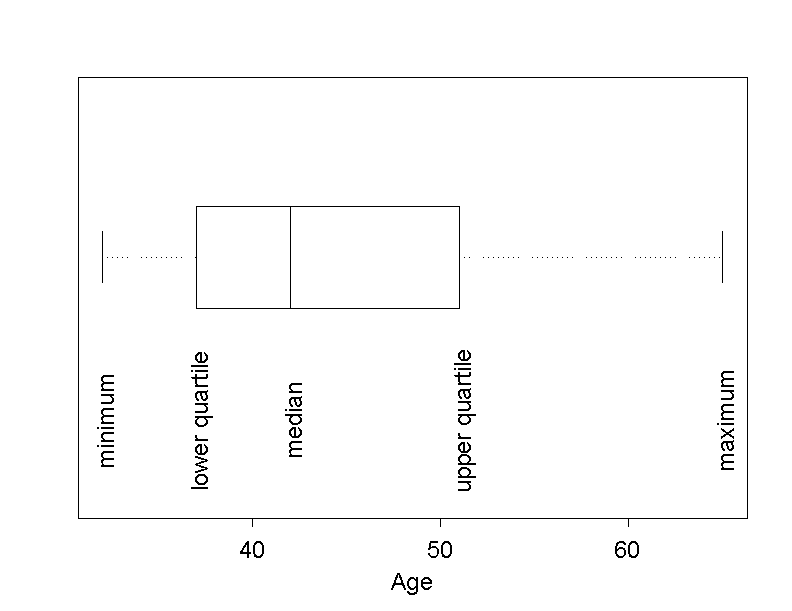
However, we cannot only read the five measures of location from this graph, but also the range and the interquartile range. The range is the distance between the two ends of the plot and the interquartile range is the length of the box.
With the help of a boxplot, it can also be assessed whether the data are distributed symmetrically or not. If the vertical line, which represents the median, divides the box into equal parts, then this is an indication for a symmetrical distribution. If the left part of the box is shorter than the right part, this indicates that the data are more widely scattered above the median than below it. In this case, we speak of a "right-skewed" distribution. In the converse situation (i.e. if the left part of the box is wider than the right part), we speak of a "left-skewed" distribution.
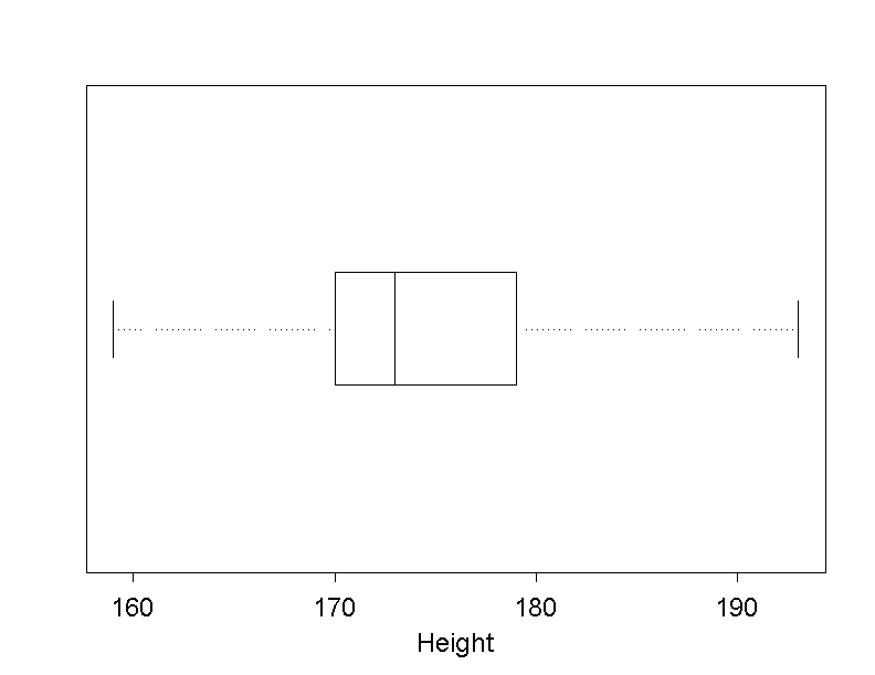
The following boxplot represents the body height of Dr. Frank N. Stein's male chemical employees.
Statistical measures (statistics) can be divided into "measures of location" and "measures of dispersion". Measures of location provide information about the location of the data.
In order to describe the centre of the data, the mean value or the median are used. If the distribution of the data is skewed, the median is generally preferred.
More general measures of location are the percentiles. The \((100 \times p)\)-th percentile divides the data into the \((100 \times p)\%\) smallest and the \((100 \times (1-p))\%\) largest values. Special cases of percentiles are the median (\(50\)-th percentile), the lower quartile (\(25\)-th percentile) and the upper quartile (\(75\)-th percentile).
Measures of dispersion describe the scatter of the data. The scatter of the data around the mean value is measured by the "standard deviation". The wider the scatter of the data around the mean value, the larger the standard deviation. Other measures of dispersion are the "interquartile range", which measures the spread of the central fifty per cent of the data and the range, which measures the spread of the whole sample.
In a boxplot, the following seven statistical measures represented: minimum, lower quartile (or \(25\)-th percentile), median, upper quartile (or \(75\)-th percentile) and maximum (measures of location), range and interquartile range (measures of dispersion). Occasionally, the mean is additionally represented as a dot.
All of these measures are only meaningful for quantitative variables. When dealing with qualitative variables, the relevant statistical measures are the relative frequencies of the different values (or categories) of the respective variables.