|
This chapter is devoted to the distribution of sample statistics (mainly of the sample mean and of an observed proportion), which represent random quantities themselves, if one considers their variation across different random samples. You will learn how the variability of the sample statistics and hence the precision of statements about the population depend on the sample size and the variation of the underlying variable. The idea of describing the accuracy of a sample estimate with an interval leads to the central statistical concept of "confidence interval". |
|
Educational objectives
You know the essential properties of sample means and other sample statistics. You are familiar with the term "standard error" and you are able to explain it in your own words. You know the law by which the standard error decreases with increasing sample size and how the distribution of the means of a quantitative variable across many large random samples from the same population can be described. You are familiar with the important concept of the "\(95\%\)-confidence interval" and can explain it in your own words. You are able to calculate \(95\%\)- confidence intervals yourself (which are valid for large sample sizes) based on sample statistics and their standard errors. You know how to construct exact confidence intervals (i.e. which are also valid for small sample sizes) for proportions (relative frequencies). Key words: sampling distribution, standard error, square root of n law, approximate normal distribution, confidence interval Previous knowledge: population (chap. 1), sample statistics (chap. 3/4), normal distribution (chap. 6), binominal distribution (chap. 7) Central questions: How can we make inferences on a population parameter based on the respective statistic from a random sample (e.g. the sample mean of the body height of men or the observed proportion of persons with hay fever) and make exact statements despite the randomness of the sample? |
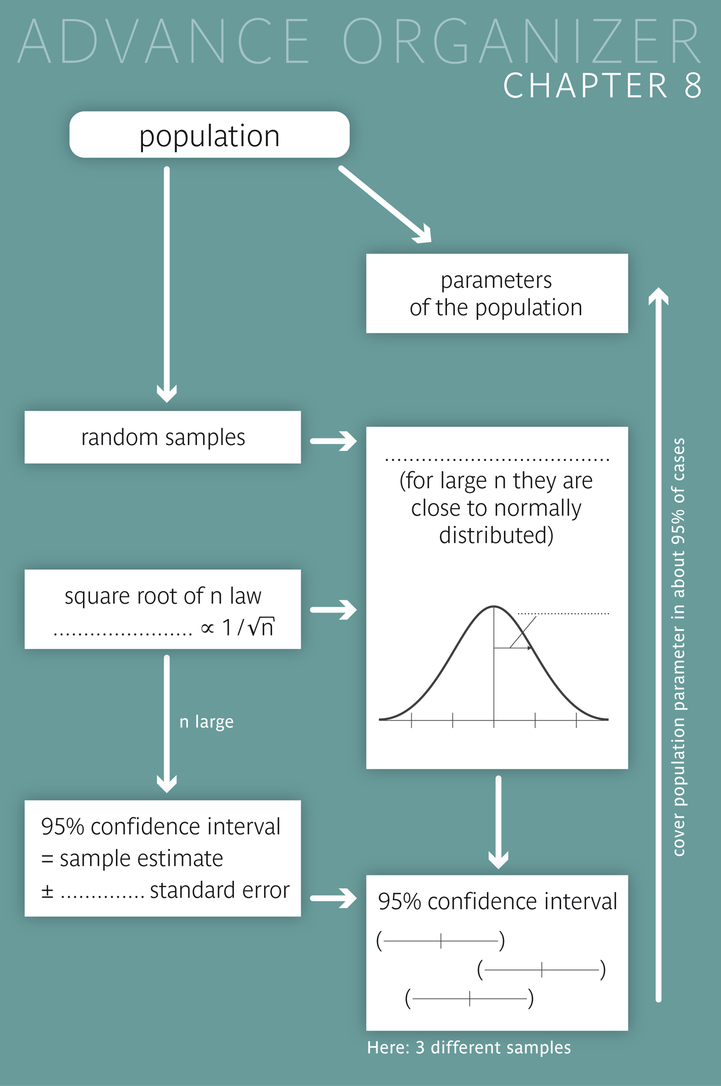
In statistics, the goal is not only to describe the data of a survey or trial in a clear and comprehensible way (descriptive statistics), but also to make inferences from the collected data on the underlying population. This is the role of so-called "inferential statistics". One of its main tasks is to provide valid statements on population parameters based on corresponding sample statistics. As we already know from chapter 4, this is only possible if the data come from a random sample. If we make inferences on a population parameter based on a sample statistic, we have to consider that these two values do not agree in general. If we take the true population parameter as a benchmark, each of its estimates from a random sample is fraught with a random error. This random error is defined as the following difference \[ \text{random error = observed statistic - population parameter} \] It is thus important to know the distribution of these random errors across different random samples of the same size from the given population. This distribution has the exact same shape as the distribution of the statistic itself, referred to as "sampling distribution" of the statistic. We could identify the sampling distribution of a statistic by drawing a larger number of random samples of the same size from the given population and calculating the statistic in each of the samples. In practice, however, this is hardly possible. Therefore we make use of the probability calculus or of artificially generated (so-called simulated) random samples from a virtual population.
You may ask yourself why "sample mean" appears in its singular form in this title. This is not a linguistic error, but should emphasise that we are talking about the sample characteristic "mean value" which varies from one sample to another, much the same as body height varies from one person to another. In the case of body height, the observational units are persons, whereas the observational units in the case of the sample mean are different random samples of the same size from a given population. We are thus interested in the distribution of the mean across all possible random samples of a certain size from a given population. In this chapter, the observational units are thus no longer single individuals, but random samples.
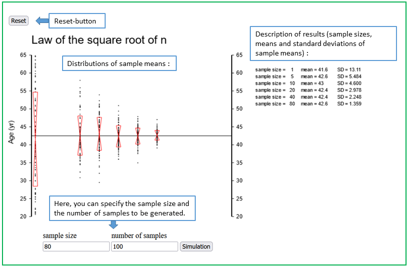
With the applet "Square root of n law* you can observe how the variability of the sample mean decreases with increasing sample size.
Exercise:
Choose \( S = 100 \) (\( \rightarrow \) entry field "number of samples") and start with \( n = 1 \) (\( \rightarrow \) entry field "sample size"). Samples of size 1 are individual observations. Therefore, the resulting figure illustrates the distribution of individual values of the respective variable. Next choose \( n = 4 \), followed by \( n = 8, n = 16, n = 32 \) and \( n = 64. \), and observe what happens to the variability of the points (now representing sample means and no longer individual values within a sample).
|
Synopsis 8.2.1
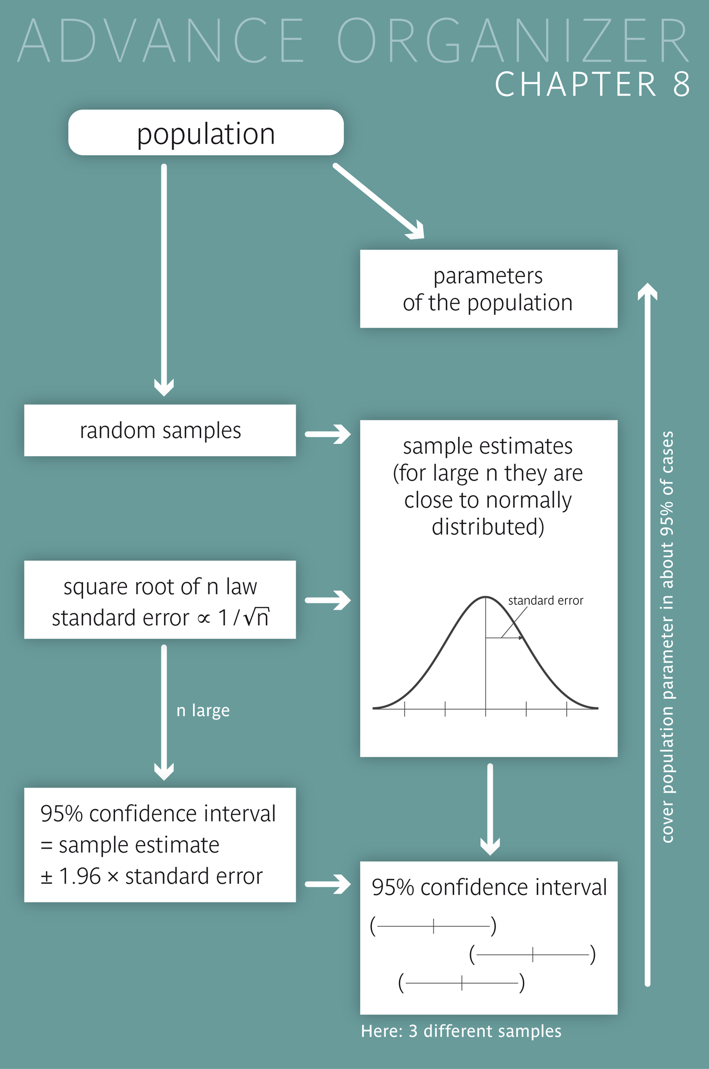
The means of random samples of the same size n from a given population have the following properties: a) The means of random samples vary around the population mean \( \mu \). b) The variability of the sample means decreases with increasing sample size \( n \). c) If the sample only represents a small fraction of the population, the standard deviation of the sample means is inversely proportional to \(\sqrt{n}\) (square root of \(n\) law) d) The standard deviation of the sample means, referred to as "standard error" (abbr. SE), satisfies \[ \text{SE} = \sigma / \sqrt{n} \] where \( \sigma \) denotes the standard deviation of the variable in the population and \( n \) the sample size. Statements b), c) and d) apply to all quantitative variables whose values cannot become arbitrarily large. |
The abbreviation SE is derived from the term "standard error". Sometimes the abbreviation SEM (standard error of the mean) is used for the standard error of the sample mean. The denominator of the formula under d) reflects the preceding statement c). Furthermore the following applies: the bigger the variability of the individual values, the bigger the variability of the sample means calculated from them. It is thus plausible that the standard deviation of the variable itself appears in the numerator. In practice, where \( \sigma \) is generally unknown - just like the population mean \(\mu \) itself -, \( \sigma \) is estimated by the standard deviation \( s \) of the variable in the observed sample.
In the preceding section you learned how the spread of the sampling distribution of the mean decreases with increasing sample size. In the
following section you will learn how the shape of the sampling distribution
of the mean changes with increasing sample size. Open the applet "Central limit theorem", which illustrates an important law of probability theory..
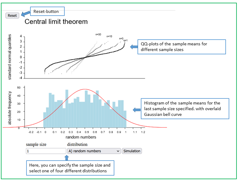
Question Nr. 8.3.1 What can you observe?
First choose the initial distribution 1), as described in the instructions of the applet
and increase the sample size gradually from 1 to 5, 10, 20, 40, 80.
How does the Q-Q plot change with increasing sample size? What does this mean? Note down your observations.
Repeat these steps for distributions 2) and 3).
How fast does the shape of the Q-Q plot change? Are there differences compared to what you observed in the first step?
We can summarise these observations in the following synopsis.
|
Synopsis 8.3.1
As long as the observed samples only represent a small fraction of the population, the following statements apply: a) The sampling distribution of the mean approaches a Gaussian bell curve with increasing sample size. b) This "convergence" of the sampling distribution of the mean to the normal distribution generally occurs relatively fast (i.e. already with relatively small sample sizes) for variables with an approximately symmetrical distribution and a Q-Q plot that does not have a pronounced S-shape. For variables with a skewed distribution or a Q-Q plot with a pronounced S-shape, larger sample sizes are required. These statements hold for all quantitative variables which cannot take arbitrarily large values. |
Statement a) summarizes one of the central laws of probability theory, which is known under the name "central limit theorem".
In chapter 6, we saw that \(95\%\) of all observations of a normally distributed variable lie in the range \( \mu \pm 1.96 \times \sigma \), where \( \mu \) and \( \sigma \) denote the mean and the standard deviation, respectively, of the variable in the underlying population. We now know that sample means are approximately normally distributed for sufficiently large sample sizes \( n \) and have a standard deviation of \[ SE = \sigma/\sqrt{n} \,\,\text{(standard error)}.\] Hence the following holds true for approx. \(95\%\) of all sample means \( \bar{x} \) from random samples of size \( n \): \[ \bar{x} \, \text{lies in the interval} \, [\mu - 1.96 \times SE, \mu + 1.96 \times SE ] .\] If we now substitute the unknown population mean \( \mu \) in the interval above with one of the concrete sample means \( \bar{x} \), we get an interval of equal width \[ [ \bar{x} - 1.96 \times SE, \, \bar{x} + 1.96 \times SE ] .\] However, this interval varies with \( \bar{x} \) from one sample to another. It has the important property that it contains the unknown population mean \( \mu \) in \(95\%\) of all samples. In other words: we can be \(95\%\) confident that this interval contains the true population mean value \( \mu \). Therefore this interval is called "\(95\%\)-confidence interval" for the population mean \( \mu \). It may not be evident that this property of the confidence interval derives directly from the first statement about the distribution of the sample means \( \bar{x} \) around \( \mu \).
Let's thus take a look at the following analogy: we compare the samples, whose mean values \( \bar{x} \) lie in the interval \( (\mu - 1.96 \times SE, \, \mu + 1.96 \times SE) \), with the number of all people whose place of domicile ( \( \sim \bar{x} \)) lies within 100 km of their place of birth (\( \sim \mu \)). The exact same group of people can say that their place of birth (\( \sim \mu \)) is within 100 km of their place of domicile ( \( \sim \bar{x} \)), i.e., that it lies within a radius of 100 km of the place of domicile (\( \sim \) confidence interval).
For math enthusiasts we also give the respective formal derivation: The statement \[ \bar{x} \, \text{lies in} \, [ \mu - 1.96 \times \sigma/\sqrt{n}, \, \mu + 1.96 \times \sigma/\sqrt{n} ] \] is equivalent to \[ \mu - 1.96 \times \sigma/\sqrt{n} \leq \bar{x} \leq \mu + 1.96 \times \sigma/\sqrt{n} .\] This inequality is now transformed as follows: We first subtract \( \mu \) in each of the three parts of the inequality and get \[ -1.96 \times \sigma/\sqrt{n} \leq \bar{x} - \mu \leq + 1.96 \times \sigma/\sqrt{n} .\] In a next step we multiply each of the three parts with (-1), which leads to an inversion of the inequalities \[ 1.96 \times \sigma/\sqrt{n} \geq \mu - \bar{x} \geq -1.96 \times \sigma/\sqrt{n} .\] Now we add \( \bar{x} \) and obtain \[ \bar{x} + 1.96 \times \sigma/\sqrt{n} \geq \mu \geq \bar{x} - 1.96 \times \sigma/\sqrt{n} .\] Expressing this with \( \leq \)-relations, we finally get \[ \bar{x} - 1.96 \times \sigma/\sqrt{n} \leq \mu \leq \bar{x} + 1.96 \times \sigma/\sqrt{n} .\] This means that the population mean \( \mu \) lies between the following two limits \[ \bar{x} - 1.96 \times \sigma/\sqrt{n} \,\, \text{and} \,\, \bar{x} + 1.96 \times \sigma/\sqrt{n} .\] Therefore, the following interval \[ [ \bar{x} - 1.96 \times \sigma/\sqrt{n}, \, \bar{x} + 1.96 \times \sigma/\sqrt{n} ] \] covers the population mean \( \mu \) in \(95\%\) of all random samples of size \( n \).
|
Definition 8.4.1
The interval \( \bar{x} \pm 1.96 \times SE \), which contains the unknown population mean \( \mu \) in 95% of all random samples, is called "\(95\%\)-confidence interval" for the population mean \( \mu \). |
|
Synopsis 8.4.1
The (unknown) population mean \( \mu \) lies in the 95%-confidence interval \[ [ \bar{x} - 1.96 \times \frac{\sigma}{\sqrt{n}}, \, \bar{x} + 1.96 \times \frac{\sigma}{\sqrt{n}} ] .\] in approx. \(95\%\) of all random samples, provided that the sample size \( n \) is large enough. For each individual interval we can be \(95\%\) confident that it contains the population mean value \( \mu \). This statement applies to all quantitative variables which cannot take arbitrarily large values. |
The applet "Confidence intervals of sample means" illustrates this important property of the confidence interval.
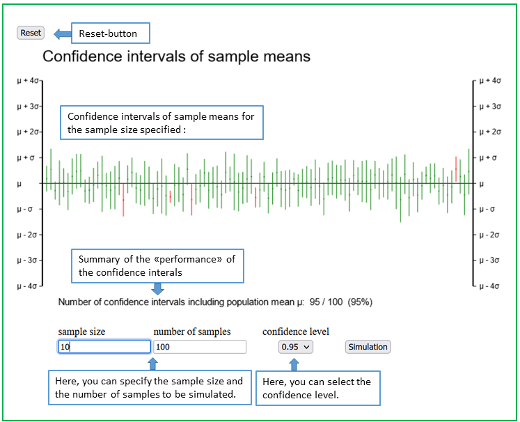
This applet illustrates the scatter of confidence intervals of sample means around the underlying population mean μ. Confidence intervals cover μ with a fixed "probability", defined by the confidence level (denoted by 1 - α). Usually, the confidence level is 0.95 (or 95%). The term probability is put in quotation marks because we do not have repeated samples in practice, and an individual confidence interval either contains μ or not. This is different if data are repeatedly simulated from a "virtual" population whose mean value μ is known. In our example, μ is represented by the horizontal line. Individual values used to compute sample means are simulated from a normal distribution with mean value μ and standard deviation σ.
You can specify the sample size n and the number S of random samples to be generated. However, n must be larger than 1 to be able to calculate confidence intervals. You can also change the confidence level using the drop down menu. If you press the key "Simulation", S confindence intervals are plotted as vertical lines with a tiny dot in the middle. These dots are the means of simulated samples of size n.
With small sample sizes, you can observe considerable variations of the lengths of the confidence intervals, because the standard deviations, from which the standard errors are estimated, vary considerably from sample to sample. If the confidence level is 1 - α, then a proportion of 1 - α of confidence intervals will on average include the underlying population mean μ. Confidence intervals including μ are represented in green color, those missing μ are red.
The coverage property of confidence intervals is independent of the sample size. This is because the width of the confidence intervals adapts to the sample size. The confidence intervals get shorter if the sample size n is increased.
This applet shows that, on average, approx. \(95\) of \(100\) samples provide a \(95\%\)-confidence interval, which contains the true population mean \( \mu \). This value, which is unknown in reality, is represented by a horizontal line. Conversely, \(5\%\) of the \(95\%\)-confidence intervals do not include \( \mu \), on average. The applet enables the choice of other confidence levels (i.e., \( 0.9 \) and \( 0.99 \)). Naturally the confidence intervals get wider with increasing and narrower with decreasing confidence level. As an alternative to the classical \(95\%\)-confidence interval, the following confidence intervals are also encountered:
The factors used with the standard error are the \(95\)th, \(99.5\)th and \(99.95\)th percentiles, respectively, of the standard normal distribution
What has been said for the sample mean also applies to many other sample statistics (median, percentiles, standard deviation, variance, interquartile range, etc.) under relatively weak additional conditions. In these cases, however, the standard error can seldom be calculated in an easy way. However, there are also sample statistics for which the statements b) to e) of the following synopsis do not hold (e.g. maximum, minimum and range).
|
Synopsis 8.4.2
In the following the symbol \( \theta \) will be used to denote the population parameter and the symbol \( \hat{\theta} \) to denote the respective sample statistic. The following statements apply: a) If different random samples are drawn, the statistic \( \hat{\theta} \) varies around the respective population parameter \( \theta \). b) The standard error SE of many statistics \( \hat{\theta} \) decreases with increasing sample size \( n \). As long as the observed samples only represent a small fraction of the population, the following additional statements apply under relatively weak conditions: c) The standard error \( SE \) of many statistics \( \hat{\theta} \) is essentially inversely proportional to the square root of the sample size \( n \). d) The sampling distribution of many statistics \( \hat{\theta} \) approaches a Gaussian bell curve around the respective population parameter \( \Theta \) with increasing sample size \( n \). Hence the following applies to such sample statistics \( \hat{\theta} \) in sufficiently large samples: e) The \(95\%\)-confidence interval \[ [\hat{\theta} - 1.96 \times SE, \, \hat{\theta} + 1.96 \times SE] \] contains the population parameter \( \Theta \) in approx. \(95\%\) of all random samples. Important: These statements only hold true for random samples. |
The calculation rule for confidence intervals of a sample mean is only accurate for large sample sizes \( n \). The standard error is generally unknown and must be estimated from the sample data using the formula \( s / \sqrt{n} \) where \( s \) denotes the standard deviation of the variable \( X \) in the sample. As \( s \) also varies from sample to sample, another random error creeps in (in addition to the one of the mean). This random error has a considerable impact in smaller samples, but loses importance with increasing sample size. For samples of size > 120 it becomes negligible. For sample sizes \( \leq 120 \) it is advisable to use a factor larger than 1.96 in the formula of the \(95\%\)-confidence interval. This factor is derived from the so-called "\(t\)- distribution" with \( n-1 \) degrees of freedom, where \( n \) again denotes the sample size. You can memorise that the number of degrees of freedom is equal to the denominator of the variance. For the \(95\%\)-confidence interval, this factor equals the \(97.5\)th percentile of the respective \(t\)-distribution. The smaller \( n \) , the wider the respective \(t\)-distribution and the larger the factor to be used.
The \(95\%\)-confidence interval for the population mean \( \mu \) is then given by \[ \bar{x} \pm t_{0.975,n-1} \times s/\sqrt{n} \] where \( t_{0.975,n-1} \) denotes the \(97.5\)th percentile of the \(t\)-distribution with \( n-1 \) degrees of freedom.
The following table gives the values of \( t_{0.975,n-1} \) for different degrees of freedom
| df = number of degrees of freedom | 97.5th percentile (\( t_{0.975,df} \)) |
|---|---|
| 5 | 2.571 |
| 10 | 2.228 |
| 20 | 2.086 |
| 50 | 2.009 |
| 100 | 1.984 |
For instance, in a random sample of \(6\) men for which the mean value and the standard deviation of the body height are \(178\) cm and \(7.5\) cm, the value \(2.571\) must be used to multiply the standard error. The \(95\%\)-confidence interval of the mean body height in the population from which this sample was drawn can be calculated based on the above formula as follows: \[ 178 \pm 2.571 \times 7.5 / \sqrt{6} = [170.1, 185.9] \]
The confidence intervals are calculated based on this formula in the applet "Confidence intervals of sample means". Since the standard deviation now also varies from one sample to another, not only the centres but also the widths of the confidence intervals display random fluctuations. This can be clearly seen if he sample size \( n \) is small. Statistics programs also use \(t\)-quantiles to calculate confidence intervals for population mean values. In the absence of a statistics program, you can use Excel to calculate \(t\)-quantiles via the function \(T.INV(q ; df)\) , where \( q = 0.975 \) for the \(95\%\)-confidence interval, \( q = 0.95 \) for the \(90\%\)-confidence interval and \( q = 0.995 \) for the \(99\%\)-confidence interval.
Dr. Frank N. Stein has read in a medical journal that a new medicine, which was recommended to him by a pharmaceutical representative, caused adverse reactions in \(18\) out of \(200\) patients during a treatment of one month. Based on this result, he estimates the probability of adverse reactions of this medicine during a one month treatment to be \(18/200 = 0.09\) or \(9\%\). He considers this value to be too high but he would consider a probability of adverse reactions of \(5\%\) as acceptable. Because he is aware of the fact that sample results are affected by random errors, he wants to calculate the \(95\%\)-confidence interval for the probability in question. To do so, he needs to know the standard error of the observed proportion of adverse reactions. (In this section, we will mostly use the term "proportion" for a relative frequency). In a statistics textbook he finds the following formula for the standard error of a proportion: \[ SE = \sqrt{\frac{p \ (1-p)} {n}} \] where \( n \) denotes the sample size and \( p \) the observed proportion.
In his case, \( n = 200 \) and \( p = 0.09 \). By inserting these values into the formula he gets \( SE = 0.0202 \). Dr. Frank N. Stein now calculates the \(95\%\)- confidence interval for the unknown probability as \( 0.09 \pm 1.96 \times 0.0202 \). This interval has a lower limit of \(0.0503\) and an upper limit of \(0.1297\). Dr. Stein can thus be \(95\%\) confident that the probability of adverse reactions lies in the interval \( [0.0503, 0.1297] \). If the probability of adverse reactions were in reality only \(5\%\) or even lower, this would represent one of the rare instances (occurrung in only \(5\%\) of all cases), in which the \(95\%\)-confidence interval does not include the true population parameter. Consequently, Dr. Stein cannot believe that adverse reactions would only occur in \(5\%\) of all patients.
For maths enthusiasts:
You might have noticed the similarity of this formula with the one of the standard deviation of the binominal distribution. An event which occurs with a probability \( \pi \) will occur on average \( n \times \pi \) times in a series of \( n \) observations, with a standard deviation of \( \sqrt{n \times \pi \times (1 - \pi)} \). The observed proportion \( p \) is obtained by dividing the number of events by \( n \). Therefore, the observed proportion will on average be \( \frac{n \times \pi}{n} = \pi \) and the standard deviation of \( p \) will be \[ \frac{ \sqrt{n \times \pi \times (1 - \pi)}} {n} = \sqrt{\frac{n \times \pi \times (1 - \pi)}{n^2} } = \sqrt{\frac{\pi \times (1 - \pi)}{n} } \] As we don't know \( \pi \), we have to replace it by its sample estimate \( p \), which provides the formula for the standard error which Dr. Stein used.
|
Synopsis 8.5.1
If a specific outcome occurs with a relative frequency \( p \) in a random sample of size \( n \), if the sample only represents a small fraction of the population and if \( n \times p \times (1 - p) \geq 10 \) holds, then a) the standard error of \( p \) can be estimated by \[ \sqrt{\frac{p \times (1 - p)}{n}} \] b) the \(95\%\)-confidence interval for the probability \( \pi \) of this outcome in the population can be approximated by \[ [ p - 1.96 \times \sqrt{\frac{p \times (1 - p)}{n}} , \, p + 1.96 \times \sqrt{\frac{p \times (1 - p)}{n}} ] .\] |
What can be done if the approximate confidence interval of an observed proportion \( p \). is not accurate enough, which is the case if \( n \times p \times (1 - p) \lt 10 \) holds (cf. chapter 7)?
With the applet to the genotype example you will learn how exact confidence intervals for an unknown probability can be constructed. To do this, we consider the following example:
A certain genotype \( G \), which is known to be associated with an increased risk of a disease \( D \), was found six times in a random sample of \(30\) people from a given population. The observed proportion of this genotype was thus \(0.2\) or \(20\%\).
With the applet "Applet to the genotype example" you can find an exact \(95\%\)-confidence interval
for \( \pi \).
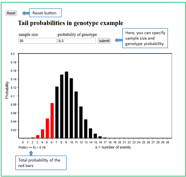
First examine what happens if you assume a value of \(0.4\) for \( \pi \)
Now suppose that \( \pi \) equals \(0.1\).
Next you can use the applet "Exact and approximate confidence intervals of proportions" to see how the number \( n \) of trials (or observational units) and the number \( m \) of observed events (or outcomes of interest) influences the shape of the exact \(95\%\)-confidence interval for the unknown probability \( \pi \) of the event (or outcome of interest in the underlying population).
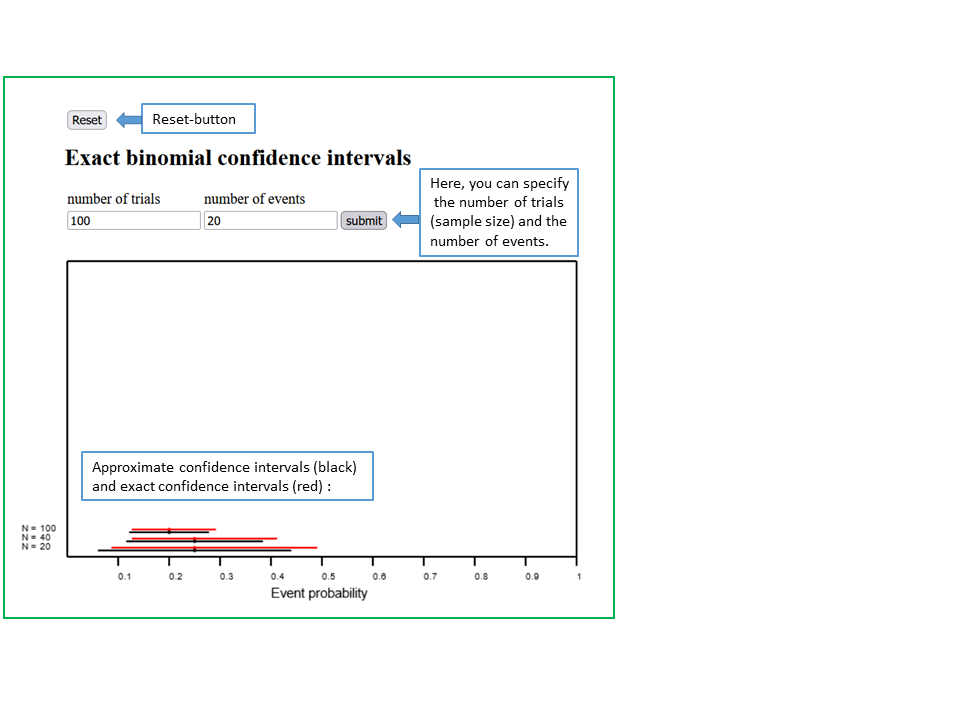
In a second step, you can also vary the proportion of observed events. In this case it is best to fix the number of trials \( n \) and to vary the number \( m \) of observed events. Ideally, \( n \) should be at least \( 40 \), as \( 40 \times \frac{m}{n} \times (1 - \frac{m}{n}) \) would otherwise be smaller than \( 10 \) for all possible choices of \( m \).
In this chapter, the observational units were no longer individual persons or objects, but random samples of persons or objects. The measures used to describe the individual samples are called sample statistics. They are used to estimate the respective unknown population parameters.
Due to chance, the sample statistics change from one sample to another. The so-called standard error (SE) is used as a measure of this variation. The size of the standard error depends on the sample size: the larger the sample size, the smaller the standard error. In fact, the standard error of a sample mean or a proportion is inversely proportional to the square root of the sample size, and this essentially also holds for many other sample statistics.
The sample size also influences the distribution of the sample statistics (i.e., the sampling distribution). For many statistics, the sampling distribution approaches a Gaussian bell curve (convergence to the normal distribution), as the sample size increases. This leads to the important concept of the confidence interval. A confidence interval for a specific parameter of the population is constructed around the respective sample statistic. Its limits are defined in such a way that they include the unknown population parameter in a pre-defined percentage of samples, usually \(95\%\). For many sample statistics, the \(95\%\)-confidence interval is computed according to the formula "\(\text{sample statistic} \pm 1.96 \times SE \)".